Note
Click here to download the full example code
Linear classifier on sensor data with plot patterns and filters
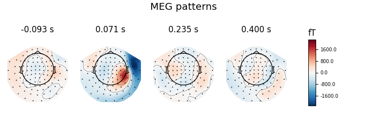
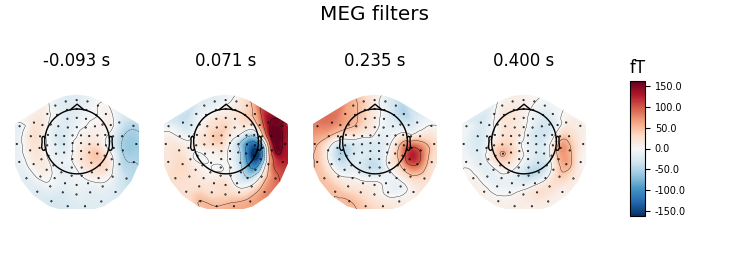
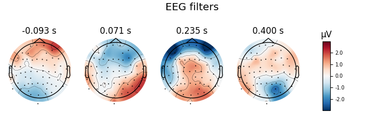
Here decoding, a.k.a MVPA or supervised machine learning, is applied to M/EEG data in sensor space. Fit a linear classifier with the LinearModel object providing topographical patterns which are more neurophysiologically interpretable 1 than the classifier filters (weight vectors). The patterns explain how the MEG and EEG data were generated from the discriminant neural sources which are extracted by the filters. Note patterns/filters in MEG data are more similar than EEG data because the noise is less spatially correlated in MEG than EEG.
# Authors: Alexandre Gramfort <alexandre.gramfort@inria.fr>
#          Romain Trachel <trachelr@gmail.com>
#          Jean-Remi King <jeanremi.king@gmail.com>
#
# License: BSD (3-clause)

import mne
from mne import io, EvokedArray
from mne.datasets import sample
from mne.decoding import Vectorizer, get_coef

from sklearn.preprocessing import StandardScaler
from sklearn.linear_model import LogisticRegression
from sklearn.pipeline import make_pipeline

# import a linear classifier from mne.decoding
from mne.decoding import LinearModel

print(__doc__)

data_path = sample.data_path()
sample_path = data_path + '/MEG/sample'
Set parameters
raw_fname = sample_path + '/sample_audvis_filt-0-40_raw.fif'
event_fname = sample_path + '/sample_audvis_filt-0-40_raw-eve.fif'
tmin, tmax = -0.1, 0.4
event_id = dict(aud_l=1, vis_l=3)

# Setup for reading the raw data
raw = io.read_raw_fif(raw_fname, preload=True)
raw.filter(.5, 25, fir_design='firwin')
events = mne.read_events(event_fname)

# Read epochs
epochs = mne.Epochs(raw, events, event_id, tmin, tmax, proj=True,
                    decim=2, baseline=None, preload=True)
del raw

labels = epochs.events[:, -1]

# get MEG and EEG data
meg_epochs = epochs.copy().pick_types(meg=True, eeg=False)
meg_data = meg_epochs.get_data().reshape(len(labels), -1)
Out:
Opening raw data file /home/circleci/mne_data/MNE-sample-data/MEG/sample/sample_audvis_filt-0-40_raw.fif...
    Read a total of 4 projection items:
        PCA-v1 (1 x 10²)  idle
        PCA-v2 (1 x 10²)  idle
        PCA-v3 (1 x 10²)  idle
        Average EEG reference (1 x 60)  idle
    Range : 6450 ... 48149 =     42.956 ...   320.665 secs
Ready.
Reading 0 ... 41699  =      0.000 ...   277.709 secs...
Filtering raw data in 1 contiguous segment
Setting up band-pass filter from 0.5 - 25 Hz

FIR filter parameters
---------------------
Designing a one-pass, zero-phase, non-causal bandpass filter:
- Windowed time-domain design (firwin) method
- Hamming window with 0.0194 passband ripple and 53 dB stopband attenuation
- Lower passband edge: 0.50
- Lower transition bandwidth: 0.50 Hz (-6 dB cutoff frequency: 0.25 Hz)
- Upper passband edge: 25.00 Hz
- Upper transition bandwidth: 6.25 Hz (-6 dB cutoff frequency: 28.12 Hz)
- Filter length: 993 samples (6.613 sec)

Not setting metadata
Not setting metadata
145 matching events found
No baseline correction applied
Created an SSP operator (subspace dimension = 4)
4 projection items activated
Loading data for 145 events and 76 original time points ...
0 bad epochs dropped
Removing projector <Projection | Average EEG reference, active : True, n_channels : 60>
Decoding in sensor space using a LogisticRegression classifier
clf = LogisticRegression(solver='lbfgs')
scaler = StandardScaler()

# create a linear model with LogisticRegression
model = LinearModel(clf)

# fit the classifier on MEG data
X = scaler.fit_transform(meg_data)
model.fit(X, labels)

# Extract and plot spatial filters and spatial patterns
for name, coef in (('patterns', model.patterns_), ('filters', model.filters_)):
    # We fitted the linear model onto Z-scored data. To make the filters
    # interpretable, we must reverse this normalization step
    coef = scaler.inverse_transform([coef])[0]

    # The data was vectorized to fit a single model across all time points and
    # all channels. We thus reshape it:
    coef = coef.reshape(len(meg_epochs.ch_names), -1)

    # Plot
    evoked = EvokedArray(coef, meg_epochs.info, tmin=epochs.tmin)
    evoked.plot_topomap(title='MEG %s' % name, time_unit='s')
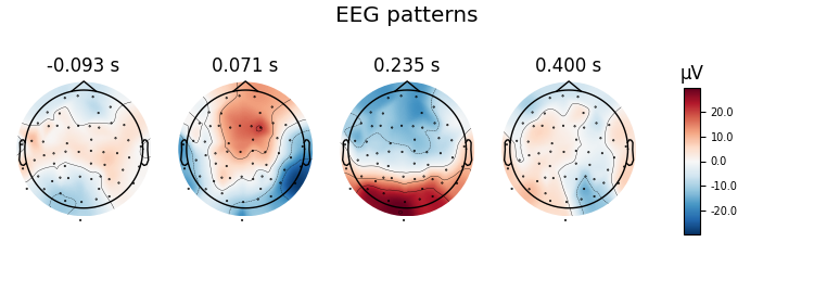
Let’s do the same on EEG data using a scikit-learn pipeline
X = epochs.pick_types(meg=False, eeg=True)
y = epochs.events[:, 2]

# Define a unique pipeline to sequentially:
clf = make_pipeline(
    Vectorizer(),                       # 1) vectorize across time and channels
    StandardScaler(),                   # 2) normalize features across trials
    LinearModel(
        LogisticRegression(solver='lbfgs')))  # 3) fits a logistic regression
clf.fit(X, y)

# Extract and plot patterns and filters
for name in ('patterns_', 'filters_'):
    # The `inverse_transform` parameter will call this method on any estimator
    # contained in the pipeline, in reverse order.
    coef = get_coef(clf, name, inverse_transform=True)
    evoked = EvokedArray(coef, epochs.info, tmin=epochs.tmin)
    evoked.plot_topomap(title='EEG %s' % name[:-1], time_unit='s')
Out:
Removing projector <Projection | PCA-v1, active : True, n_channels : 102>
Removing projector <Projection | PCA-v2, active : True, n_channels : 102>
Removing projector <Projection | PCA-v3, active : True, n_channels : 102>
References
- 1
Stefan Haufe, Frank Meinecke, Kai Görgen, Sven Dähne, John-Dylan Haynes, Benjamin Blankertz, and Felix Bießmann. On the interpretation of weight vectors of linear models in multivariate neuroimaging. NeuroImage, 87:96–110, 2014. doi:10.1016/j.neuroimage.2013.10.067.
Total running time of the script: ( 0 minutes 5.176 seconds)
Estimated memory usage: 1033 MB