Note
Click here to download the full example code
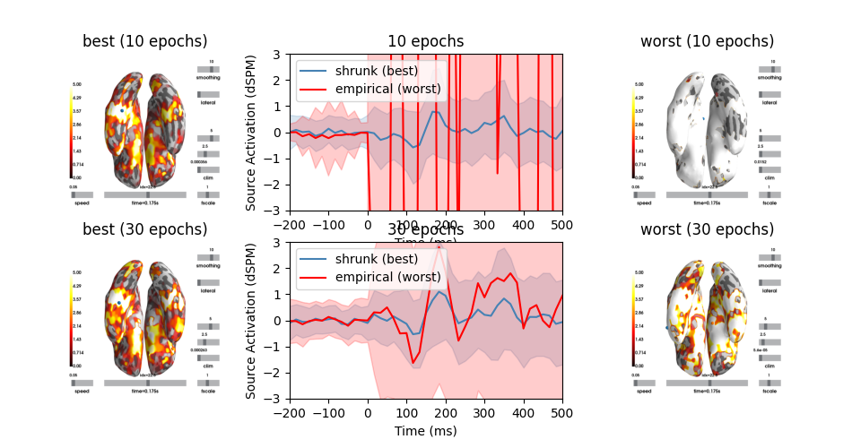
Demonstrate impact of whitening on source estimates
This example demonstrates the relationship between the noise covariance estimate and the MNE / dSPM source amplitudes. It computes source estimates for the SPM faces data and compares proper regularization with insufficient regularization based on the methods described in 1. This example demonstrates that improper regularization can lead to overestimation of source amplitudes. This example makes use of the previous, non-optimized code path that was used before implementing the suggestions presented in 1.
This example does quite a bit of processing, so even on a fast machine it can take a couple of minutes to complete.
Warning
Please do not copy the patterns presented here for your own analysis, this is example is purely illustrative.
# Author: Denis A. Engemann <denis.engemann@gmail.com>
#
# License: BSD (3-clause)

import numpy as np
import matplotlib.pyplot as plt

import mne
from mne import io
from mne.datasets import spm_face
from mne.minimum_norm import apply_inverse, make_inverse_operator
from mne.cov import compute_covariance

print(__doc__)
Get data
data_path = spm_face.data_path()
subjects_dir = data_path + '/subjects'

raw_fname = data_path + '/MEG/spm/SPM_CTF_MEG_example_faces%d_3D.ds'

raw = io.read_raw_ctf(raw_fname % 1)  # Take first run
# To save time and memory for this demo, we'll just use the first
# 2.5 minutes (all we need to get 30 total events) and heavily
# resample 480->60 Hz (usually you wouldn't do either of these!)
raw.crop(0, 150.).pick_types(meg=True, stim=True, exclude='bads').load_data()
raw.filter(None, 20.)

events = mne.find_events(raw, stim_channel='UPPT001')

event_ids = {"faces": 1, "scrambled": 2}
tmin, tmax = -0.2, 0.5
baseline = (None, 0)
reject = dict(mag=3e-12)

# inverse parameters
conditions = 'faces', 'scrambled'
snr = 3.0
lambda2 = 1.0 / snr ** 2
clim = dict(kind='value', lims=[0, 2.5, 5])
Out:
ds directory : /home/circleci/mne_data/MNE-spm-face/MEG/spm/SPM_CTF_MEG_example_faces1_3D.ds
    res4 data read.
    hc data read.
    Separate EEG position data file not present.
    Quaternion matching (desired vs. transformed):
      -0.90   72.01    0.00 mm <->   -0.90   72.01   -0.00 mm (orig :  -43.09   61.46 -252.17 mm) diff =    0.000 mm
       0.90  -72.01    0.00 mm <->    0.90  -72.01   -0.00 mm (orig :   53.49  -45.24 -258.02 mm) diff =    0.000 mm
      98.30    0.00    0.00 mm <->   98.30   -0.00    0.00 mm (orig :   78.60   72.16 -241.87 mm) diff =    0.000 mm
    Coordinate transformations established.
    Polhemus data for 3 HPI coils added
    Device coordinate locations for 3 HPI coils added
    Measurement info composed.
Finding samples for /home/circleci/mne_data/MNE-spm-face/MEG/spm/SPM_CTF_MEG_example_faces1_3D.ds/SPM_CTF_MEG_example_faces1_3D.meg4:
    System clock channel is available, checking which samples are valid.
    1 x 324474 = 324474 samples from 340 chs
Current compensation grade : 3
Reading 0 ... 72000  =      0.000 ...   150.000 secs...
Filtering raw data in 1 contiguous segment
Setting up low-pass filter at 20 Hz

FIR filter parameters
---------------------
Designing a one-pass, zero-phase, non-causal lowpass filter:
- Windowed time-domain design (firwin) method
- Hamming window with 0.0194 passband ripple and 53 dB stopband attenuation
- Upper passband edge: 20.00 Hz
- Upper transition bandwidth: 5.00 Hz (-6 dB cutoff frequency: 22.50 Hz)
- Filter length: 317 samples (0.660 sec)

41 events found
Event IDs: [1 2 3]
Estimate covariances
samples_epochs = 5, 15,
method = 'empirical', 'shrunk'
colors = 'steelblue', 'red'
epochs = mne.Epochs(
    raw, events, event_ids, tmin, tmax,
    baseline=baseline, preload=True, reject=reject, decim=8)
del raw

noise_covs = list()
evokeds = list()
stcs = list()
methods_ordered = list()
for n_train in samples_epochs:
    # estimate covs based on a subset of samples
    # make sure we have the same number of conditions.
    idx = np.sort(np.concatenate([
        np.where(epochs.events[:, 2] == event_ids[cond])[0][:n_train]
        for cond in conditions]))
    epochs_train = epochs[idx]
    epochs_train.equalize_event_counts(event_ids)
    assert len(epochs_train) == 2 * n_train

    # We know some of these have too few samples, so suppress warning
    # with verbose='error'
    noise_covs.append(compute_covariance(
        epochs_train, method=method, tmin=None, tmax=0,  # baseline only
        return_estimators=True, rank=None, verbose='error'))  # returns list
    # prepare contrast
    evokeds.append([epochs_train[k].average() for k in conditions])
    del epochs_train
del epochs

# Make forward
trans = data_path + '/MEG/spm/SPM_CTF_MEG_example_faces1_3D_raw-trans.fif'
# oct5 and add_dist are just for speed, not recommended in general!
src = mne.setup_source_space(
    'spm', spacing='oct5', subjects_dir=data_path + '/subjects',
    add_dist=False)
bem = data_path + '/subjects/spm/bem/spm-5120-5120-5120-bem-sol.fif'
forward = mne.make_forward_solution(evokeds[0][0].info, trans, src, bem)
del src
for noise_covs_, evokeds_ in zip(noise_covs, evokeds):
    # do contrast

    # We skip empirical rank estimation that we introduced in response to
    # the findings in reference [1] to use the naive code path that
    # triggered the behavior described in [1]. The expected true rank is
    # 274 for this dataset. Please do not do this with your data but
    # rely on the default rank estimator that helps regularizing the
    # covariance.
    stcs.append(list())
    methods_ordered.append(list())
    for cov in noise_covs_:
        inverse_operator = make_inverse_operator(
            evokeds_[0].info, forward, cov, loose=0.2, depth=0.8)
        assert len(inverse_operator['sing']) == 274  # sanity check
        stc_a, stc_b = (apply_inverse(e, inverse_operator, lambda2, "dSPM",
                                      pick_ori=None) for e in evokeds_)
        stc = stc_a - stc_b
        methods_ordered[-1].append(cov['method'])
        stcs[-1].append(stc)
    del inverse_operator, cov, stc, stc_a, stc_b
del forward, noise_covs, evokeds  # save some memory
Out:
Not setting metadata
Not setting metadata
37 matching events found
Applying baseline correction (mode: mean)
0 projection items activated
Loading data for 37 events and 337 original time points ...
0 bad epochs dropped
Dropped 0 epochs:
Dropped 0 epochs:
Setting up the source space with the following parameters:

SUBJECTS_DIR = /home/circleci/mne_data/MNE-spm-face/subjects
Subject      = spm
Surface      = white
Octahedron subdivision grade 5

>>> 1. Creating the source space...

Doing the octahedral vertex picking...
Loading /home/circleci/mne_data/MNE-spm-face/subjects/spm/surf/lh.white...
Mapping lh spm -> oct (5) ...
    Triangle neighbors and vertex normals...
Loading geometry from /home/circleci/mne_data/MNE-spm-face/subjects/spm/surf/lh.sphere...
Setting up the triangulation for the decimated surface...
loaded lh.white 1026/139164 selected to source space (oct = 5)

Loading /home/circleci/mne_data/MNE-spm-face/subjects/spm/surf/rh.white...
Mapping rh spm -> oct (5) ...
    Triangle neighbors and vertex normals...
Loading geometry from /home/circleci/mne_data/MNE-spm-face/subjects/spm/surf/rh.sphere...
Setting up the triangulation for the decimated surface...
loaded rh.white 1026/137848 selected to source space (oct = 5)

You are now one step closer to computing the gain matrix
Source space          : <SourceSpaces: [<surface (lh), n_vertices=139164, n_used=1026>, <surface (rh), n_vertices=137848, n_used=1026>] MRI (surface RAS) coords, subject 'spm', ~21.2 MB>
MRI -> head transform : /home/circleci/mne_data/MNE-spm-face/MEG/spm/SPM_CTF_MEG_example_faces1_3D_raw-trans.fif
Measurement data      : instance of Info
Conductor model   : /home/circleci/mne_data/MNE-spm-face/subjects/spm/bem/spm-5120-5120-5120-bem-sol.fif
Accurate field computations
Do computations in head coordinates
Free source orientations

Read 2 source spaces a total of 2052 active source locations

Coordinate transformation: MRI (surface RAS) -> head
     0.999622  0.006802  0.026647      -2.80 mm
    -0.014131  0.958276  0.285497       6.72 mm
    -0.023593 -0.285765  0.958009       9.43 mm
     0.000000  0.000000  0.000000       1.00

Read 274 MEG channels from info
Read  29 MEG compensation channels from info
99 coil definitions read
Coordinate transformation: MEG device -> head
     0.997940 -0.049681 -0.040594      -1.35 mm
     0.054745  0.989330  0.135013      -0.41 mm
     0.033453 -0.136957  0.990012      65.80 mm
     0.000000  0.000000  0.000000       1.00
5 compensation data sets in info
MEG coil definitions created in head coordinates.
Removing 5 compensators from info because not all compensation channels were picked.
Source spaces are now in head coordinates.

Setting up the BEM model using /home/circleci/mne_data/MNE-spm-face/subjects/spm/bem/spm-5120-5120-5120-bem-sol.fif...

Loading surfaces...

Loading the solution matrix...

Three-layer model surfaces loaded.
Loaded linear_collocation BEM solution from /home/circleci/mne_data/MNE-spm-face/subjects/spm/bem/spm-5120-5120-5120-bem-sol.fif
Employing the head->MRI coordinate transform with the BEM model.
BEM model spm-5120-5120-5120-bem-sol.fif is now set up

Source spaces are in head coordinates.
Checking that the sources are inside the surface (will take a few...)
    Skipping interior check for 422 sources that fit inside a sphere of radius   52.6 mm
    Skipping solid angle check for 0 points using Qhull
    Skipping interior check for 424 sources that fit inside a sphere of radius   52.6 mm
    Skipping solid angle check for 0 points using Qhull

Setting up compensation data...
    274 out of 274 channels have the compensation set.
    Desired compensation data (3) found.
    All compensation channels found.
    Preselector created.
    Compensation data matrix created.
    Postselector created.

Composing the field computation matrix...
Composing the field computation matrix (compensation coils)...
Computing MEG at 2052 source locations (free orientations)...

Finished.
Converting forward solution to surface orientation
    No patch info available. The standard source space normals will be employed in the rotation to the local surface coordinates....
    Converting to surface-based source orientations...
    [done]
Computing inverse operator with 274 channels.
    274 out of 274 channels remain after picking
Removing 5 compensators from info because not all compensation channels were picked.
Selected 274 channels
Creating the depth weighting matrix...
    274 magnetometer or axial gradiometer channels
    limit = 2030/2052 = 10.151735
    scale = 3.95792e-11 exp = 0.8
Applying loose dipole orientations to surface source spaces: 0.2
Whitening the forward solution.
Removing 5 compensators from info because not all compensation channels were picked.
Computing rank from covariance with rank=None
    Using tolerance 4.5e-14 (2.2e-16 eps * 274 dim * 0.74  max singular value)
    Estimated rank (mag): 130
    MAG: rank 130 computed from 274 data channels with 0 projectors
    Setting small MAG eigenvalues to zero (without PCA)
Creating the source covariance matrix
Adjusting source covariance matrix.
Computing SVD of whitened and weighted lead field matrix.
    largest singular value = 3.90845
    scaling factor to adjust the trace = 6.13275e+18
Removing 5 compensators from info because not all compensation channels were picked.
Preparing the inverse operator for use...
    Scaled noise and source covariance from nave = 1 to nave = 5
    Created the regularized inverter
    The projection vectors do not apply to these channels.
    Created the whitener using a noise covariance matrix with rank 130 (144 small eigenvalues omitted)
    Computing noise-normalization factors (dSPM)...
[done]
Applying inverse operator to "faces"...
    Picked 274 channels from the data
    Computing inverse...
    Eigenleads need to be weighted ...
    Computing residual...
    Explained  91.8% variance
    Combining the current components...
    dSPM...
[done]
Removing 5 compensators from info because not all compensation channels were picked.
Preparing the inverse operator for use...
    Scaled noise and source covariance from nave = 1 to nave = 5
    Created the regularized inverter
    The projection vectors do not apply to these channels.
    Created the whitener using a noise covariance matrix with rank 130 (144 small eigenvalues omitted)
    Computing noise-normalization factors (dSPM)...
[done]
Applying inverse operator to "scrambled"...
    Picked 274 channels from the data
    Computing inverse...
    Eigenleads need to be weighted ...
    Computing residual...
    Explained  91.6% variance
    Combining the current components...
    dSPM...
[done]
Converting forward solution to surface orientation
    No patch info available. The standard source space normals will be employed in the rotation to the local surface coordinates....
    Converting to surface-based source orientations...
    [done]
Computing inverse operator with 274 channels.
    274 out of 274 channels remain after picking
Removing 5 compensators from info because not all compensation channels were picked.
Selected 274 channels
Creating the depth weighting matrix...
    274 magnetometer or axial gradiometer channels
    limit = 2030/2052 = 10.151735
    scale = 3.95792e-11 exp = 0.8
Applying loose dipole orientations to surface source spaces: 0.2
Whitening the forward solution.
Removing 5 compensators from info because not all compensation channels were picked.
Computing rank from covariance with rank=None
    Using tolerance 4.6e-14 (2.2e-16 eps * 274 dim * 0.76  max singular value)
    Estimated rank (mag): 130
    MAG: rank 130 computed from 274 data channels with 0 projectors
    Setting small MAG eigenvalues to zero (without PCA)
Creating the source covariance matrix
Adjusting source covariance matrix.
Computing SVD of whitened and weighted lead field matrix.
    largest singular value = 5.08889
    scaling factor to adjust the trace = 5.47473e+22
Removing 5 compensators from info because not all compensation channels were picked.
Preparing the inverse operator for use...
    Scaled noise and source covariance from nave = 1 to nave = 5
    Created the regularized inverter
    The projection vectors do not apply to these channels.
    Created the whitener using a noise covariance matrix with rank 130 (144 small eigenvalues omitted)
    Computing noise-normalization factors (dSPM)...
[done]
Applying inverse operator to "faces"...
    Picked 274 channels from the data
    Computing inverse...
    Eigenleads need to be weighted ...
    Computing residual...
    Explained  99.7% variance
    Combining the current components...
    dSPM...
[done]
Removing 5 compensators from info because not all compensation channels were picked.
Preparing the inverse operator for use...
    Scaled noise and source covariance from nave = 1 to nave = 5
    Created the regularized inverter
    The projection vectors do not apply to these channels.
    Created the whitener using a noise covariance matrix with rank 130 (144 small eigenvalues omitted)
    Computing noise-normalization factors (dSPM)...
[done]
Applying inverse operator to "scrambled"...
    Picked 274 channels from the data
    Computing inverse...
    Eigenleads need to be weighted ...
    Computing residual...
    Explained  99.6% variance
    Combining the current components...
    dSPM...
[done]
Converting forward solution to surface orientation
    No patch info available. The standard source space normals will be employed in the rotation to the local surface coordinates....
    Converting to surface-based source orientations...
    [done]
Computing inverse operator with 274 channels.
    274 out of 274 channels remain after picking
Removing 5 compensators from info because not all compensation channels were picked.
Selected 274 channels
Creating the depth weighting matrix...
    274 magnetometer or axial gradiometer channels
    limit = 2030/2052 = 10.151735
    scale = 3.95792e-11 exp = 0.8
Applying loose dipole orientations to surface source spaces: 0.2
Whitening the forward solution.
Removing 5 compensators from info because not all compensation channels were picked.
Computing rank from covariance with rank=None
    Using tolerance 3.7e-14 (2.2e-16 eps * 274 dim * 0.61  max singular value)
    Estimated rank (mag): 274
    MAG: rank 274 computed from 274 data channels with 0 projectors
    Setting small MAG eigenvalues to zero (without PCA)
Creating the source covariance matrix
Adjusting source covariance matrix.
Computing SVD of whitened and weighted lead field matrix.
    largest singular value = 4.11868
    scaling factor to adjust the trace = 5.99801e+18
Removing 5 compensators from info because not all compensation channels were picked.
Preparing the inverse operator for use...
    Scaled noise and source covariance from nave = 1 to nave = 15
    Created the regularized inverter
    The projection vectors do not apply to these channels.
    Created the whitener using a noise covariance matrix with rank 274 (0 small eigenvalues omitted)
    Computing noise-normalization factors (dSPM)...
[done]
Applying inverse operator to "faces"...
    Picked 274 channels from the data
    Computing inverse...
    Eigenleads need to be weighted ...
    Computing residual...
    Explained  86.6% variance
    Combining the current components...
    dSPM...
[done]
Removing 5 compensators from info because not all compensation channels were picked.
Preparing the inverse operator for use...
    Scaled noise and source covariance from nave = 1 to nave = 15
    Created the regularized inverter
    The projection vectors do not apply to these channels.
    Created the whitener using a noise covariance matrix with rank 274 (0 small eigenvalues omitted)
    Computing noise-normalization factors (dSPM)...
[done]
Applying inverse operator to "scrambled"...
    Picked 274 channels from the data
    Computing inverse...
    Eigenleads need to be weighted ...
    Computing residual...
    Explained  86.9% variance
    Combining the current components...
    dSPM...
[done]
Converting forward solution to surface orientation
    No patch info available. The standard source space normals will be employed in the rotation to the local surface coordinates....
    Converting to surface-based source orientations...
    [done]
Computing inverse operator with 274 channels.
    274 out of 274 channels remain after picking
Removing 5 compensators from info because not all compensation channels were picked.
Selected 274 channels
Creating the depth weighting matrix...
    274 magnetometer or axial gradiometer channels
    limit = 2030/2052 = 10.151735
    scale = 3.95792e-11 exp = 0.8
Applying loose dipole orientations to surface source spaces: 0.2
Whitening the forward solution.
Removing 5 compensators from info because not all compensation channels were picked.
Computing rank from covariance with rank=None
    Using tolerance 3.9e-14 (2.2e-16 eps * 274 dim * 0.63  max singular value)
    Estimated rank (mag): 274
    MAG: rank 274 computed from 274 data channels with 0 projectors
    Setting small MAG eigenvalues to zero (without PCA)
Creating the source covariance matrix
Adjusting source covariance matrix.
Computing SVD of whitened and weighted lead field matrix.
    largest singular value = 5.40023
    scaling factor to adjust the trace = 5.55091e+19
Removing 5 compensators from info because not all compensation channels were picked.
Preparing the inverse operator for use...
    Scaled noise and source covariance from nave = 1 to nave = 15
    Created the regularized inverter
    The projection vectors do not apply to these channels.
    Created the whitener using a noise covariance matrix with rank 274 (0 small eigenvalues omitted)
    Computing noise-normalization factors (dSPM)...
[done]
Applying inverse operator to "faces"...
    Picked 274 channels from the data
    Computing inverse...
    Eigenleads need to be weighted ...
    Computing residual...
    Explained  93.1% variance
    Combining the current components...
    dSPM...
[done]
Removing 5 compensators from info because not all compensation channels were picked.
Preparing the inverse operator for use...
    Scaled noise and source covariance from nave = 1 to nave = 15
    Created the regularized inverter
    The projection vectors do not apply to these channels.
    Created the whitener using a noise covariance matrix with rank 274 (0 small eigenvalues omitted)
    Computing noise-normalization factors (dSPM)...
[done]
Applying inverse operator to "scrambled"...
    Picked 274 channels from the data
    Computing inverse...
    Eigenleads need to be weighted ...
    Computing residual...
    Explained  93.2% variance
    Combining the current components...
    dSPM...
[done]
Show the resulting source estimates
fig, (axes1, axes2) = plt.subplots(2, 3, figsize=(9.5, 5))

for ni, (n_train, axes) in enumerate(zip(samples_epochs, (axes1, axes2))):
    # compute stc based on worst and best
    ax_dynamics = axes[1]
    for stc, ax, method, kind, color in zip(stcs[ni],
                                            axes[::2],
                                            methods_ordered[ni],
                                            ['best', 'worst'],
                                            colors):
        brain = stc.plot(subjects_dir=subjects_dir, hemi='both', clim=clim,
                         initial_time=0.175, background='w', foreground='k')
        brain.show_view('ven')
        im = brain.screenshot()
        brain.close()

        ax.axis('off')
        ax.get_xaxis().set_visible(False)
        ax.get_yaxis().set_visible(False)
        ax.imshow(im)
        ax.set_title('{0} ({1} epochs)'.format(kind, n_train * 2))

        # plot spatial mean
        stc_mean = stc.data.mean(0)
        ax_dynamics.plot(stc.times * 1e3, stc_mean,
                         label='{0} ({1})'.format(method, kind),
                         color=color)
        # plot spatial std
        stc_var = stc.data.std(0)
        ax_dynamics.fill_between(stc.times * 1e3, stc_mean - stc_var,
                                 stc_mean + stc_var, alpha=0.2, color=color)

    # signal dynamics worst and best
    ax_dynamics.set(title='{0} epochs'.format(n_train * 2),
                    xlabel='Time (ms)', ylabel='Source Activation (dSPM)',
                    xlim=(tmin * 1e3, tmax * 1e3), ylim=(-3, 3))
    ax_dynamics.legend(loc='upper left', fontsize=10)

fig.subplots_adjust(hspace=0.2, left=0.01, right=0.99, wspace=0.03)
References
- 1(1,2)
Denis A. Engemann and Alexandre Gramfort. Automated model selection in covariance estimation and spatial whitening of MEG and EEG signals. NeuroImage, 108:328–342, 2015. doi:10.1016/j.neuroimage.2014.12.040.
Total running time of the script: ( 0 minutes 53.315 seconds)
Estimated memory usage: 876 MB