Note
Click here to download the full example code
Compute source power using DICS beamformer
Compute a Dynamic Imaging of Coherent Sources (DICS) 1 filter from single-trial activity to estimate source power across a frequency band. This example demonstrates how to source localize the event-related synchronization (ERS) of beta band activity in this dataset: Somatosensory
# Author: Marijn van Vliet <w.m.vanvliet@gmail.com>
#         Roman Goj <roman.goj@gmail.com>
#         Denis Engemann <denis.engemann@gmail.com>
#         Stefan Appelhoff <stefan.appelhoff@mailbox.org>
#
# License: BSD (3-clause)
import os.path as op

import numpy as np
import mne
from mne.datasets import somato
from mne.time_frequency import csd_morlet
from mne.beamformer import make_dics, apply_dics_csd

print(__doc__)
Reading the raw data and creating epochs:
data_path = somato.data_path()
subject = '01'
task = 'somato'
raw_fname = op.join(data_path, 'sub-{}'.format(subject), 'meg',
                    'sub-{}_task-{}_meg.fif'.format(subject, task))

# Use a shorter segment of raw just for speed here
raw = mne.io.read_raw_fif(raw_fname)
raw.crop(0, 120)  # one minute for speed (looks similar to using all ~800 sec)

# Read epochs
events = mne.find_events(raw)

epochs = mne.Epochs(raw, events, event_id=1, tmin=-1.5, tmax=2, preload=True)
del raw

# Paths to forward operator and FreeSurfer subject directory
fname_fwd = op.join(data_path, 'derivatives', 'sub-{}'.format(subject),
                    'sub-{}_task-{}-fwd.fif'.format(subject, task))
subjects_dir = op.join(data_path, 'derivatives', 'freesurfer', 'subjects')
Out:
Opening raw data file /home/circleci/mne_data/MNE-somato-data/sub-01/meg/sub-01_task-somato_meg.fif...
    Range : 237600 ... 506999 =    791.189 ...  1688.266 secs
Ready.
15 events found
Event IDs: [1]
Not setting metadata
Not setting metadata
15 matching events found
Applying baseline correction (mode: mean)
0 projection items activated
Loading data for 15 events and 1052 original time points ...
0 bad epochs dropped
We are interested in the beta band. Define a range of frequencies, using a log scale, from 12 to 30 Hz.
freqs = np.logspace(np.log10(12), np.log10(30), 9)
Computing the cross-spectral density matrix for the beta frequency band, for different time intervals. We use a decim value of 20 to speed up the computation in this example at the loss of accuracy.
csd = csd_morlet(epochs, freqs, tmin=-1, tmax=1.5, decim=20)
csd_baseline = csd_morlet(epochs, freqs, tmin=-1, tmax=0, decim=20)
# ERS activity starts at 0.5 seconds after stimulus onset
csd_ers = csd_morlet(epochs, freqs, tmin=0.5, tmax=1.5, decim=20)
info = epochs.info
del epochs
Out:
Computing cross-spectral density from epochs...
    Computing CSD matrix for epoch 1
    Computing CSD matrix for epoch 2
    Computing CSD matrix for epoch 3
    Computing CSD matrix for epoch 4
    Computing CSD matrix for epoch 5
    Computing CSD matrix for epoch 6
    Computing CSD matrix for epoch 7
    Computing CSD matrix for epoch 8
    Computing CSD matrix for epoch 9
    Computing CSD matrix for epoch 10
    Computing CSD matrix for epoch 11
    Computing CSD matrix for epoch 12
    Computing CSD matrix for epoch 13
    Computing CSD matrix for epoch 14
    Computing CSD matrix for epoch 15
[done]
To compute the source power for a frequency band, rather than each frequency separately, we average the CSD objects across frequencies.
csd = csd.mean()
csd_baseline = csd_baseline.mean()
csd_ers = csd_ers.mean()
Computing DICS spatial filters using the CSD that was computed on the entire timecourse.
fwd = mne.read_forward_solution(fname_fwd)
filters = make_dics(info, fwd, csd, noise_csd=csd_baseline,
                    pick_ori='max-power', reduce_rank=True)
del fwd
Out:
Reading forward solution from /home/circleci/mne_data/MNE-somato-data/derivatives/sub-01/sub-01_task-somato-fwd.fif...
    Reading a source space...
    [done]
    Reading a source space...
    [done]
    2 source spaces read
    Desired named matrix (kind = 3523) not available
    Read MEG forward solution (8155 sources, 306 channels, free orientations)
    Source spaces transformed to the forward solution coordinate frame
Identifying common channels ...
Dropped the following channels:
['STI 001', 'STI 014', 'STI 004', 'STI 016', 'EOG 061', 'STI 005', 'STI 003', 'STI 015', 'STI 006', 'STI 002']
Identifying common channels ...
Computing inverse operator with 306 channels.
    306 out of 306 channels remain after picking
Selected 306 channels
Creating the depth weighting matrix...
Whitening the forward solution.
Computing rank from covariance with rank=None
    Using tolerance 3.2e-14 (2.2e-16 eps * 306 dim * 0.47  max singular value)
    Estimated rank (mag + grad): 64
    MEG: rank 64 computed from 306 data channels with 0 projectors
    Setting small MEG eigenvalues to zero (without PCA)
Creating the source covariance matrix
Adjusting source covariance matrix.
Computing DICS spatial filters...
Computing beamformer filters for 8155 sources
Filter computation complete
Applying DICS spatial filters separately to the CSD computed using the baseline and the CSD computed during the ERS activity.
Out:
Computing DICS source power...
[done]
Computing DICS source power...
[done]
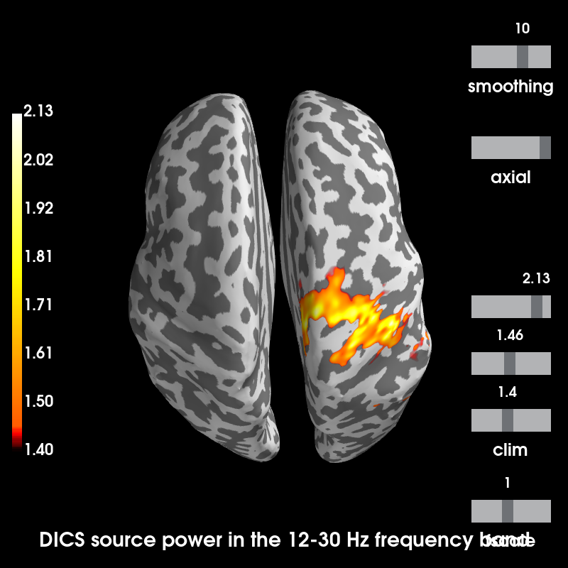
Visualizing source power during ERS activity relative to the baseline power.
stc = beta_source_power / baseline_source_power
message = 'DICS source power in the 12-30 Hz frequency band'
brain = stc.plot(hemi='both', views='axial', subjects_dir=subjects_dir,
                 subject=subject, time_label=message)
Out:
Using control points [1.40049468 1.45553894 2.12583448]
References
- 1
Joachim Groß, Jan Kujala, Matti S. Hämäläinen, Lars Timmermann, Alfons Schnitzler, and Riitta Salmelin. Dynamic imaging of coherent sources: studying neural interactions in the human brain. Proceedings of the National Academy of Sciences, 98(2):694–699, 2001. doi:10.1073/pnas.98.2.694.
Total running time of the script: ( 0 minutes 17.613 seconds)
Estimated memory usage: 450 MB