Generate a functional label from source estimates

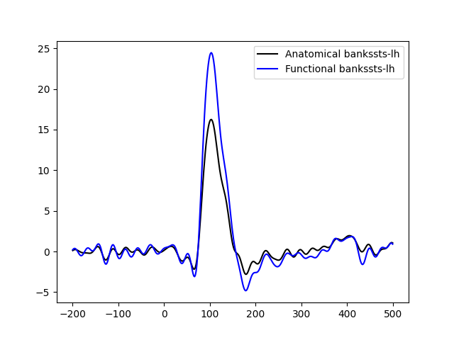
Threshold source estimates and produce a functional label. The label is typically the region of interest that contains high values. Here we compare the average time course in the anatomical label obtained by FreeSurfer segmentation and the average time course from the functional label. As expected the time course in the functional label yields higher values.

# Author: Luke Bloy <luke.bloy@gmail.com>
#         Alex Gramfort <alexandre.gramfort@inria.fr>
# License: BSD (3-clause)

import numpy as np
import matplotlib.pyplot as plt

import mne
from mne.minimum_norm import read_inverse_operator, apply_inverse
from mne.datasets import sample

print(__doc__)

data_path = sample.data_path()
fname_inv = data_path + '/MEG/sample/sample_audvis-meg-oct-6-meg-inv.fif'
fname_evoked = data_path + '/MEG/sample/sample_audvis-ave.fif'
subjects_dir = data_path + '/subjects'
subject = 'sample'

snr = 3.0
lambda2 = 1.0 / snr ** 2
method = "dSPM"  # use dSPM method (could also be MNE or sLORETA)

# Compute a label/ROI based on the peak power between 80 and 120 ms.
# The label bankssts-lh is used for the comparison.
aparc_label_name = 'bankssts-lh'
tmin, tmax = 0.080, 0.120

# Load data
evoked = mne.read_evokeds(fname_evoked, condition=0, baseline=(None, 0))
inverse_operator = read_inverse_operator(fname_inv)
src = inverse_operator['src']  # get the source space

# Compute inverse solution
stc = apply_inverse(evoked, inverse_operator, lambda2, method,
                    pick_ori='normal')

# Make an STC in the time interval of interest and take the mean
stc_mean = stc.copy().crop(tmin, tmax).mean()

# use the stc_mean to generate a functional label
# region growing is halted at 60% of the peak value within the
# anatomical label / ROI specified by aparc_label_name
label = mne.read_labels_from_annot(subject, parc='aparc',
                                   subjects_dir=subjects_dir,
                                   regexp=aparc_label_name)[0]
stc_mean_label = stc_mean.in_label(label)
data = np.abs(stc_mean_label.data)
stc_mean_label.data[data < 0.6 * np.max(data)] = 0.

# 8.5% of original source space vertices were omitted during forward
# calculation, suppress the warning here with verbose='error'
func_labels, _ = mne.stc_to_label(stc_mean_label, src=src, smooth=True,
                                  subjects_dir=subjects_dir, connected=True,
                                  verbose='error')

# take first as func_labels are ordered based on maximum values in stc
func_label = func_labels[0]

# load the anatomical ROI for comparison
anat_label = mne.read_labels_from_annot(subject, parc='aparc',
                                        subjects_dir=subjects_dir,
                                        regexp=aparc_label_name)[0]

# extract the anatomical time course for each label
stc_anat_label = stc.in_label(anat_label)
pca_anat = stc.extract_label_time_course(anat_label, src, mode='pca_flip')[0]

stc_func_label = stc.in_label(func_label)
pca_func = stc.extract_label_time_course(func_label, src, mode='pca_flip')[0]

# flip the pca so that the max power between tmin and tmax is positive
pca_anat *= np.sign(pca_anat[np.argmax(np.abs(pca_anat))])
pca_func *= np.sign(pca_func[np.argmax(np.abs(pca_anat))])

Out:

Reading /home/circleci/mne_data/MNE-sample-data/MEG/sample/sample_audvis-ave.fif ...
    Read a total of 4 projection items:
        PCA-v1 (1 x 102) active
        PCA-v2 (1 x 102) active
        PCA-v3 (1 x 102) active
        Average EEG reference (1 x 60) active
    Found the data of interest:
        t =    -199.80 ...     499.49 ms (Left Auditory)
        0 CTF compensation matrices available
        nave = 55 - aspect type = 100
Projections have already been applied. Setting proj attribute to True.
Applying baseline correction (mode: mean)
Reading inverse operator decomposition from /home/circleci/mne_data/MNE-sample-data/MEG/sample/sample_audvis-meg-oct-6-meg-inv.fif...
    Reading inverse operator info...
    [done]
    Reading inverse operator decomposition...
    [done]
    305 x 305 full covariance (kind = 1) found.
    Read a total of 4 projection items:
        PCA-v1 (1 x 102) active
        PCA-v2 (1 x 102) active
        PCA-v3 (1 x 102) active
        Average EEG reference (1 x 60) active
    Noise covariance matrix read.
    22494 x 22494 diagonal covariance (kind = 2) found.
    Source covariance matrix read.
    22494 x 22494 diagonal covariance (kind = 6) found.
    Orientation priors read.
    22494 x 22494 diagonal covariance (kind = 5) found.
    Depth priors read.
    Did not find the desired covariance matrix (kind = 3)
    Reading a source space...
    Computing patch statistics...
    Patch information added...
    Distance information added...
    [done]
    Reading a source space...
    Computing patch statistics...
    Patch information added...
    Distance information added...
    [done]
    2 source spaces read
    Read a total of 4 projection items:
        PCA-v1 (1 x 102) active
        PCA-v2 (1 x 102) active
        PCA-v3 (1 x 102) active
        Average EEG reference (1 x 60) active
    Source spaces transformed to the inverse solution coordinate frame
Preparing the inverse operator for use...
    Scaled noise and source covariance from nave = 1 to nave = 55
    Created the regularized inverter
    Created an SSP operator (subspace dimension = 3)
    Created the whitener using a noise covariance matrix with rank 302 (3 small eigenvalues omitted)
    Computing noise-normalization factors (dSPM)...
[done]
Applying inverse operator to "Left Auditory"...
    Picked 305 channels from the data
    Computing inverse...
    Eigenleads need to be weighted ...
    Computing residual...
    Explained  59.4% variance
    dSPM...
[done]
Reading labels from parcellation...
   read 1 labels from /home/circleci/mne_data/MNE-sample-data/subjects/sample/label/lh.aparc.annot
   read 0 labels from /home/circleci/mne_data/MNE-sample-data/subjects/sample/label/rh.aparc.annot
Reading labels from parcellation...
   read 1 labels from /home/circleci/mne_data/MNE-sample-data/subjects/sample/label/lh.aparc.annot
   read 0 labels from /home/circleci/mne_data/MNE-sample-data/subjects/sample/label/rh.aparc.annot
Extracting time courses for 1 labels (mode: pca_flip)
Extracting time courses for 1 labels (mode: pca_flip)

plot the time courses….

plt.figure()
plt.plot(1e3 * stc_anat_label.times, pca_anat, 'k',
         label='Anatomical %s' % aparc_label_name)
plt.plot(1e3 * stc_func_label.times, pca_func, 'b',
         label='Functional %s' % aparc_label_name)
plt.legend()
plt.show()

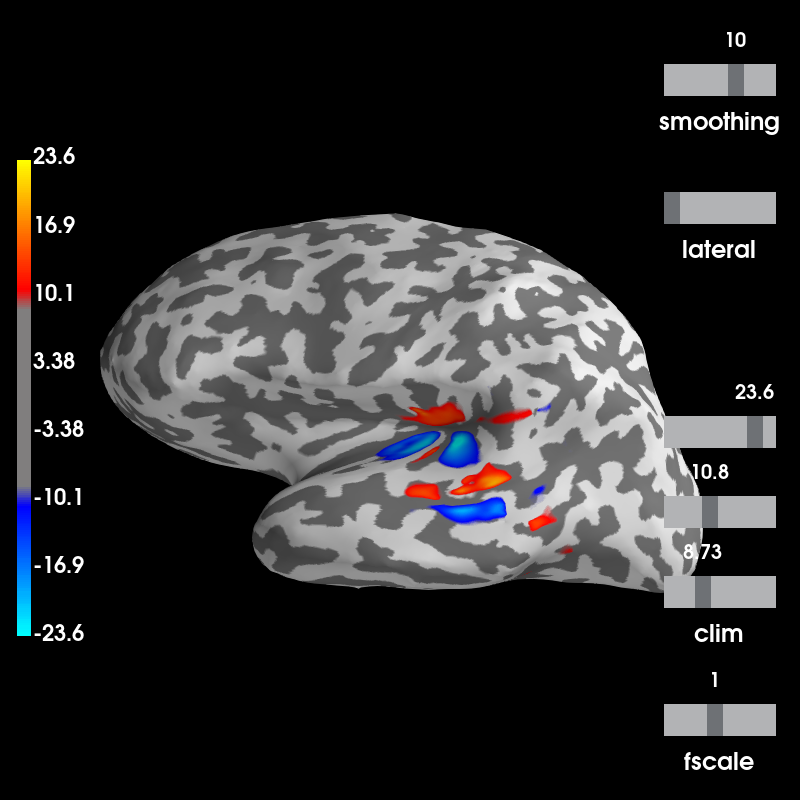
plot brain in 3D with PySurfer if available

brain = stc_mean.plot(hemi='lh', subjects_dir=subjects_dir)
brain.show_view('lateral')

# show both labels
brain.add_label(anat_label, borders=True, color='k')
brain.add_label(func_label, borders=True, color='b')

Out:

Using control points [ 8.73227205 10.80078852 23.62750681]

Estimated memory usage: 33 MB