Note
Click here to download the full example code
Morph volumetric source estimate
This example demonstrates how to morph an individual subject’s
mne.VolSourceEstimate to a common reference space. We achieve this
using mne.SourceMorph. Pre-computed data will be morphed based on
an affine transformation and a nonlinear registration method
known as Symmetric Diffeomorphic Registration (SDR) by
1.
Transformation is estimated from the subject’s anatomical T1 weighted MRI (brain) to FreeSurfer’s ‘fsaverage’ T1 weighted MRI (brain).
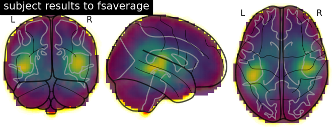
Afterwards the transformation will be applied to the volumetric source estimate. The result will be plotted, showing the fsaverage T1 weighted anatomical MRI, overlaid with the morphed volumetric source estimate.
# Author: Tommy Clausner <tommy.clausner@gmail.com>
#
# License: BSD (3-clause)
import os

import nibabel as nib
import mne
from mne.datasets import sample, fetch_fsaverage
from mne.minimum_norm import apply_inverse, read_inverse_operator
from nilearn.plotting import plot_glass_brain

print(__doc__)
Setup paths
sample_dir_raw = sample.data_path()
sample_dir = os.path.join(sample_dir_raw, 'MEG', 'sample')
subjects_dir = os.path.join(sample_dir_raw, 'subjects')

fname_evoked = os.path.join(sample_dir, 'sample_audvis-ave.fif')
fname_inv = os.path.join(sample_dir, 'sample_audvis-meg-vol-7-meg-inv.fif')

fname_t1_fsaverage = os.path.join(subjects_dir, 'fsaverage', 'mri',
                                  'brain.mgz')
fetch_fsaverage(subjects_dir)  # ensure fsaverage src exists
fname_src_fsaverage = subjects_dir + '/fsaverage/bem/fsaverage-vol-5-src.fif'
Out:
10 files missing from /home/circleci/project/mne/datasets/_fsaverage/root.txt in /home/circleci/mne_data/MNE-sample-data/subjects
Downloading missing files remotely
Downloading https://files.osf.io/v1/resources/rxvq7/providers/osfstorage/5cbdba4ef2be3c0019091890?revision=2&action=download&direct&version=2 (186.7 MB)

  0%|          | Downloading : 0.00/187M [00:00<?,        ?B/s]
  0%|          | Downloading : 504k/187M [00:00<00:06,    29.0MB/s]
  1%|1         | Downloading : 1.99M/187M [00:00<00:06,    30.1MB/s]
  2%|2         | Downloading : 3.99M/187M [00:00<00:06,    31.2MB/s]
  3%|3         | Downloading : 5.99M/187M [00:00<00:06,    30.4MB/s]
  5%|4         | Downloading : 8.99M/187M [00:00<00:05,    31.6MB/s]
  6%|5         | Downloading : 11.0M/187M [00:00<00:05,    32.8MB/s]
  7%|6         | Downloading : 13.0M/187M [00:00<00:05,    34.0MB/s]
  8%|8         | Downloading : 15.0M/187M [00:00<00:05,    35.1MB/s]
  9%|9         | Downloading : 17.0M/187M [00:00<00:04,    36.2MB/s]
 10%|#         | Downloading : 19.0M/187M [00:00<00:04,    37.5MB/s]
 11%|#1        | Downloading : 21.0M/187M [00:00<00:04,    38.8MB/s]
 14%|#4        | Downloading : 27.0M/187M [00:00<00:04,    40.5MB/s]
 17%|#6        | Downloading : 31.0M/187M [00:00<00:03,    42.0MB/s]
 19%|#8        | Downloading : 35.0M/187M [00:00<00:03,    43.5MB/s]
 21%|##        | Downloading : 39.0M/187M [00:00<00:03,    45.1MB/s]
 23%|##3       | Downloading : 43.0M/187M [00:00<00:03,    46.6MB/s]
 25%|##5       | Downloading : 47.0M/187M [00:00<00:03,    48.1MB/s]
 27%|##7       | Downloading : 51.0M/187M [00:00<00:02,    49.8MB/s]
 29%|##9       | Downloading : 55.0M/187M [00:00<00:02,    51.6MB/s]
 32%|###1      | Downloading : 59.0M/187M [00:00<00:02,    53.2MB/s]
 34%|###3      | Downloading : 63.0M/187M [00:00<00:02,    54.8MB/s]
 36%|###5      | Downloading : 67.0M/187M [00:00<00:02,    56.9MB/s]
 38%|###8      | Downloading : 71.0M/187M [00:00<00:02,    58.7MB/s]
 40%|####      | Downloading : 75.0M/187M [00:00<00:01,    60.6MB/s]
 42%|####2     | Downloading : 79.0M/187M [00:00<00:01,    62.6MB/s]
 44%|####4     | Downloading : 83.0M/187M [00:00<00:01,    65.0MB/s]
 47%|####6     | Downloading : 87.0M/187M [00:00<00:01,    66.9MB/s]
 49%|####8     | Downloading : 91.0M/187M [00:00<00:01,    69.0MB/s]
 51%|#####     | Downloading : 95.0M/187M [00:00<00:01,    70.2MB/s]
 53%|#####3    | Downloading : 99.0M/187M [00:00<00:01,    72.0MB/s]
 55%|#####5    | Downloading : 103M/187M [00:00<00:01,    74.1MB/s]
 57%|#####7    | Downloading : 107M/187M [00:00<00:01,    76.0MB/s]
 59%|#####9    | Downloading : 111M/187M [00:00<00:01,    76.7MB/s]
 62%|######1   | Downloading : 115M/187M [00:00<00:00,    78.2MB/s]
 64%|######3   | Downloading : 119M/187M [00:01<00:00,    78.9MB/s]
 66%|######5   | Downloading : 123M/187M [00:01<00:00,    79.6MB/s]
 68%|######8   | Downloading : 127M/187M [00:01<00:00,    79.7MB/s]
 70%|#######   | Downloading : 131M/187M [00:01<00:00,    80.6MB/s]
 72%|#######2  | Downloading : 135M/187M [00:01<00:00,    81.6MB/s]
 74%|#######4  | Downloading : 139M/187M [00:01<00:00,    82.8MB/s]
 77%|#######6  | Downloading : 143M/187M [00:01<00:00,    84.2MB/s]
 79%|#######8  | Downloading : 147M/187M [00:01<00:00,    85.0MB/s]
 81%|########  | Downloading : 151M/187M [00:01<00:00,    86.9MB/s]
 83%|########3 | Downloading : 155M/187M [00:01<00:00,    88.7MB/s]
 85%|########5 | Downloading : 159M/187M [00:01<00:00,    90.4MB/s]
 87%|########7 | Downloading : 163M/187M [00:01<00:00,    92.1MB/s]
 89%|########9 | Downloading : 167M/187M [00:01<00:00,    93.9MB/s]
 92%|#########1| Downloading : 171M/187M [00:01<00:00,    95.0MB/s]
 94%|#########3| Downloading : 175M/187M [00:01<00:00,    95.1MB/s]
 96%|#########5| Downloading : 179M/187M [00:01<00:00,    95.9MB/s]
 98%|#########8| Downloading : 183M/187M [00:01<00:00,    97.7MB/s]
100%|##########| Downloading : 187M/187M [00:01<00:00,    99.3MB/s]
100%|##########| Downloading : 187M/187M [00:01<00:00,     121MB/s]
Verifying hash 5133fe92b7b8f03ae19219d5f46e4177.
File saved as /tmp/tmphc9ccazo/temp.zip.

Extracting missing files
Successfully extracted 10 files
10 files missing from /home/circleci/project/mne/datasets/_fsaverage/bem.txt in /home/circleci/mne_data/MNE-sample-data/subjects/fsaverage
Downloading missing files remotely
Downloading https://files.osf.io/v1/resources/rxvq7/providers/osfstorage/5cbdb9f5353c58001aa02025?revision=4&action=download&direct&version=4 (227.8 MB)

  0%|          | Downloading : 0.00/228M [00:00<?,        ?B/s]
  0%|          | Downloading : 248k/228M [00:00<00:15,    15.7MB/s]
  0%|          | Downloading : 0.99M/228M [00:00<00:14,    16.2MB/s]
  2%|1         | Downloading : 4.49M/228M [00:00<00:13,    16.9MB/s]
  4%|3         | Downloading : 8.49M/228M [00:00<00:13,    17.5MB/s]
  5%|4         | Downloading : 10.5M/228M [00:00<00:12,    18.3MB/s]
  5%|5         | Downloading : 12.5M/228M [00:00<00:11,    19.1MB/s]
  6%|6         | Downloading : 14.5M/228M [00:00<00:11,    19.9MB/s]
  8%|8         | Downloading : 18.5M/228M [00:00<00:10,    20.8MB/s]
  9%|8         | Downloading : 20.5M/228M [00:00<00:10,    21.7MB/s]
 10%|9         | Downloading : 22.5M/228M [00:00<00:09,    22.6MB/s]
 11%|#         | Downloading : 24.5M/228M [00:00<00:09,    23.5MB/s]
 12%|#1        | Downloading : 26.5M/228M [00:00<00:08,    24.5MB/s]
 13%|#3        | Downloading : 30.5M/228M [00:00<00:08,    25.5MB/s]
 14%|#4        | Downloading : 32.5M/228M [00:00<00:07,    26.5MB/s]
 16%|#6        | Downloading : 36.5M/228M [00:00<00:07,    27.6MB/s]
 17%|#6        | Downloading : 38.5M/228M [00:00<00:06,    28.7MB/s]
 18%|#7        | Downloading : 40.5M/228M [00:00<00:06,    29.8MB/s]
 20%|#9        | Downloading : 44.5M/228M [00:00<00:06,    31.0MB/s]
 20%|##        | Downloading : 46.5M/228M [00:00<00:05,    32.2MB/s]
 21%|##1       | Downloading : 48.5M/228M [00:00<00:05,    33.4MB/s]
 22%|##2       | Downloading : 50.5M/228M [00:00<00:05,    34.7MB/s]
 23%|##3       | Downloading : 52.5M/228M [00:00<00:05,    36.0MB/s]
 24%|##3       | Downloading : 54.5M/228M [00:00<00:04,    37.3MB/s]
 25%|##4       | Downloading : 56.5M/228M [00:00<00:04,    38.5MB/s]
 27%|##6       | Downloading : 60.5M/228M [00:00<00:04,    40.0MB/s]
 27%|##7       | Downloading : 62.5M/228M [00:00<00:04,    41.4MB/s]
 28%|##8       | Downloading : 64.5M/228M [00:00<00:04,    42.6MB/s]
 29%|##9       | Downloading : 66.5M/228M [00:00<00:04,    41.6MB/s]
 30%|###       | Downloading : 68.5M/228M [00:00<00:03,    42.8MB/s]
 31%|###       | Downloading : 70.5M/228M [00:00<00:03,    44.2MB/s]
 32%|###1      | Downloading : 72.5M/228M [00:00<00:03,    45.6MB/s]
 33%|###2      | Downloading : 74.5M/228M [00:00<00:03,    47.1MB/s]
 34%|###3      | Downloading : 76.5M/228M [00:00<00:03,    48.6MB/s]
 35%|###5      | Downloading : 80.5M/228M [00:00<00:03,    50.2MB/s]
 36%|###6      | Downloading : 82.5M/228M [00:00<00:02,    51.3MB/s]
 38%|###7      | Downloading : 86.5M/228M [00:00<00:02,    52.9MB/s]
 39%|###8      | Downloading : 88.5M/228M [00:00<00:02,    54.0MB/s]
 41%|####1     | Downloading : 94.5M/228M [00:00<00:02,    55.7MB/s]
 43%|####3     | Downloading : 98.5M/228M [00:00<00:02,    56.8MB/s]
 45%|####5     | Downloading : 102M/228M [00:01<00:02,    57.5MB/s]
 47%|####6     | Downloading : 106M/228M [00:01<00:02,    58.4MB/s]
 49%|####8     | Downloading : 110M/228M [00:01<00:02,    59.5MB/s]
 50%|#####     | Downloading : 114M/228M [00:01<00:01,    60.9MB/s]
 52%|#####2    | Downloading : 118M/228M [00:01<00:01,    62.6MB/s]
 54%|#####3    | Downloading : 122M/228M [00:01<00:01,    64.2MB/s]
 56%|#####5    | Downloading : 126M/228M [00:01<00:01,    66.1MB/s]
 57%|#####7    | Downloading : 130M/228M [00:01<00:01,    68.3MB/s]
 59%|#####9    | Downloading : 134M/228M [00:01<00:01,    70.1MB/s]
 61%|######    | Downloading : 138M/228M [00:01<00:01,    71.9MB/s]
 63%|######2   | Downloading : 142M/228M [00:01<00:01,    73.3MB/s]
 64%|######4   | Downloading : 146M/228M [00:01<00:01,    74.2MB/s]
 66%|######6   | Downloading : 150M/228M [00:01<00:01,    74.3MB/s]
 68%|######7   | Downloading : 154M/228M [00:01<00:01,    72.7MB/s]
 70%|######9   | Downloading : 158M/228M [00:01<00:00,    74.3MB/s]
 71%|#######1  | Downloading : 162M/228M [00:01<00:00,    75.1MB/s]
 73%|#######3  | Downloading : 166M/228M [00:01<00:00,    77.1MB/s]
 75%|#######4  | Downloading : 170M/228M [00:01<00:00,    78.0MB/s]
 77%|#######6  | Downloading : 174M/228M [00:01<00:00,    79.3MB/s]
 78%|#######8  | Downloading : 178M/228M [00:01<00:00,    80.4MB/s]
 80%|########  | Downloading : 182M/228M [00:01<00:00,    82.4MB/s]
 82%|########1 | Downloading : 186M/228M [00:01<00:00,    83.8MB/s]
 84%|########3 | Downloading : 190M/228M [00:01<00:00,    85.2MB/s]
 85%|########5 | Downloading : 194M/228M [00:01<00:00,    86.5MB/s]
 87%|########7 | Downloading : 198M/228M [00:01<00:00,    87.4MB/s]
 89%|########8 | Downloading : 202M/228M [00:01<00:00,    88.8MB/s]
 91%|######### | Downloading : 206M/228M [00:02<00:00,    89.4MB/s]
 92%|#########2| Downloading : 210M/228M [00:02<00:00,    88.8MB/s]
 94%|#########4| Downloading : 214M/228M [00:02<00:00,    89.3MB/s]
 96%|#########5| Downloading : 218M/228M [00:02<00:00,    90.6MB/s]
 98%|#########7| Downloading : 222M/228M [00:02<00:00,    91.2MB/s]
 99%|#########9| Downloading : 226M/228M [00:02<00:00,    91.8MB/s]
100%|##########| Downloading : 228M/228M [00:02<00:00,     106MB/s]
Verifying hash b31509cdcf7908af6a83dc5ee8f49fb1.
File saved as /tmp/tmp22fge8kk/temp.zip.

Extracting missing files
Successfully extracted 10 files
Compute example data. For reference see Compute MNE-dSPM inverse solution on evoked data in volume source space
Load data:
evoked = mne.read_evokeds(fname_evoked, condition=0, baseline=(None, 0))
inverse_operator = read_inverse_operator(fname_inv)

# Apply inverse operator
stc = apply_inverse(evoked, inverse_operator, 1.0 / 3.0 ** 2, "dSPM")

# To save time
stc.crop(0.09, 0.09)
Out:
Reading /home/circleci/mne_data/MNE-sample-data/MEG/sample/sample_audvis-ave.fif ...
    Read a total of 4 projection items:
        PCA-v1 (1 x 10²) active
        PCA-v2 (1 x 10²) active
        PCA-v3 (1 x 10²) active
        Average EEG reference (1 x 60) active
    Found the data of interest:
        t =    -199.80 ...     499.49 ms (Left Auditory)
        0 CTF compensation matrices available
        nave = 55 - aspect type = 100
Projections have already been applied. Setting proj attribute to True.
Applying baseline correction (mode: mean)
Reading inverse operator decomposition from /home/circleci/mne_data/MNE-sample-data/MEG/sample/sample_audvis-meg-vol-7-meg-inv.fif...
    Reading inverse operator info...
    [done]
    Reading inverse operator decomposition...
    [done]
    305 x 305 full covariance (kind = 1) found.
    Read a total of 4 projection items:
        PCA-v1 (1 x 10²) active
        PCA-v2 (1 x 10²) active
        PCA-v3 (1 x 10²) active
        Average EEG reference (1 x 60) active
    Noise covariance matrix read.
    11271 x 11271 diagonal covariance (kind = 2) found.
    Source covariance matrix read.
    Did not find the desired covariance matrix (kind = 6)
    11271 x 11271 diagonal covariance (kind = 5) found.
    Depth priors read.
    Did not find the desired covariance matrix (kind = 3)
    Reading a source space...
    [done]
    1 source spaces read
    Read a total of 4 projection items:
        PCA-v1 (1 x 10²) active
        PCA-v2 (1 x 10²) active
        PCA-v3 (1 x 10²) active
        Average EEG reference (1 x 60) active
    Source spaces transformed to the inverse solution coordinate frame
Preparing the inverse operator for use...
    Scaled noise and source covariance from nave = 1 to nave = 55
    Created the regularized inverter
    Created an SSP operator (subspace dimension = 3)
    Created the whitener using a noise covariance matrix with rank 302 (3 small eigenvalues omitted)
    Computing noise-normalization factors (dSPM)...
[done]
Applying inverse operator to "Left Auditory"...
    Picked 305 channels from the data
    Computing inverse...
    Eigenleads need to be weighted ...
    Computing residual...
    Explained  59.7% variance
    Combining the current components...
    dSPM...
[done]
Get a SourceMorph object for VolSourceEstimate
subject_from can typically be inferred from
src,
and subject_to is set to ‘fsaverage’ by default. subjects_dir can be
None when set in the environment. In that case SourceMorph can be initialized
taking src as only argument. See mne.SourceMorph for more
details.
The default parameter setting for zooms will cause the reference volumes to be resliced before computing the transform. A value of ‘5’ would cause the function to reslice to an isotropic voxel size of 5 mm. The higher this value the less accurate but faster the computation will be.
The recommended way to use this is to morph to a specific destination source
space so that different subject_from morphs will go to the same space.`
A standard usage for volumetric data reads:
src_fs = mne.read_source_spaces(fname_src_fsaverage)
morph = mne.compute_source_morph(
    inverse_operator['src'], subject_from='sample', subjects_dir=subjects_dir,
    niter_affine=[10, 10, 5], niter_sdr=[10, 10, 5],  # just for speed
    src_to=src_fs, verbose=True)
Out:
    Reading a source space...
    [done]
    1 source spaces read
Volume source space(s) present...
    Loading /home/circleci/mne_data/MNE-sample-data/subjects/sample/mri/brain.mgz as "from" volume
    Loading /home/circleci/mne_data/MNE-sample-data/subjects/fsaverage/mri/brain.mgz as "to" volume
Computing nonlinear Symmetric Diffeomorphic Registration...
Optimizing translation:
    Optimizing level 2 [max iter: 10]
    Optimizing level 1 [max iter: 10]
    Optimizing level 0 [max iter: 5]
Optimizing rigid-body:
    Optimizing level 2 [max iter: 10]
    Optimizing level 1 [max iter: 10]
    Optimizing level 0 [max iter: 5]
    Translation:   22.7 mm
    Rotation:      20.7°
    R²:            96.5%
Optimizing full affine:
    Optimizing level 2 [max iter: 10]
    Optimizing level 1 [max iter: 10]
    Optimizing level 0 [max iter: 5]
    R²:            96.9%
Optimizing SDR:
    R²:            99.0%
[done]
Apply morph to VolSourceEstimate
The morph can be applied to the source estimate data, by giving it as the
first argument to the morph.apply() method:
Convert morphed VolSourceEstimate into NIfTI
We can convert our morphed source estimate into a NIfTI volume using
morph.apply(..., output='nifti1').
# Create mri-resolution volume of results
img_fsaverage = morph.apply(stc, mri_resolution=2, output='nifti1')
Plot results
# Load fsaverage anatomical image
t1_fsaverage = nib.load(fname_t1_fsaverage)

# Plot glass brain (change to plot_anat to display an overlaid anatomical T1)
display = plot_glass_brain(t1_fsaverage,
                           title='subject results to fsaverage',
                           draw_cross=False,
                           annotate=True)

# Add functional data as overlay
display.add_overlay(img_fsaverage, alpha=0.75)
Reading and writing SourceMorph from and to disk
An instance of SourceMorph can be saved, by calling
morph.save.
This methods allows for specification of a filename under which the morph
will be save in “.h5” format. If no file extension is provided, “-morph.h5”
will be appended to the respective defined filename:
>>> morph.save('my-file-name')
Reading a saved source morph can be achieved by using
mne.read_source_morph():
>>> morph = mne.read_source_morph('my-file-name-morph.h5')
Once the environment is set up correctly, no information such as
subject_from or subjects_dir must be provided, since it can be
inferred from the data and used morph to ‘fsaverage’ by default, e.g.:
>>> morph.apply(stc)
References
- 1
Brian B. Avants, Charles L. Epstein, Murray C. Grossman, and James C. Gee. Symmetric diffeomorphic image registration with cross-correlation: evaluating automated labeling of elderly and neurodegenerative brain. Medical Image Analysis, 12(1):26–41, 2008. doi:10.1016/j.media.2007.06.004.
Total running time of the script: ( 0 minutes 22.114 seconds)
Estimated memory usage: 739 MB