Plotting topographic arrowmaps of evoked data

Load evoked data and plot arrowmaps along with the topomap for selected time points. An arrowmap is based upon the Hosaka-Cohen transformation and represents an estimation of the current flow underneath the MEG sensors. They are a poor man’s MNE.

See 1 for details.

References

1

David Cohen and Hidehiro Hosaka. Part II magnetic field produced by a current dipole. Journal of Electrocardiology, 9(4):409–417, 1976. doi:10.1016/S0022-0736(76)80041-6.

# Authors: Sheraz Khan <sheraz@khansheraz.com>
#
# License: BSD (3-clause)

import numpy as np
import mne
from mne.datasets import sample
from mne.datasets.brainstorm import bst_raw
from mne import read_evokeds
from mne.viz import plot_arrowmap

print(__doc__)

path = sample.data_path()
fname = path + '/MEG/sample/sample_audvis-ave.fif'

# load evoked data
condition = 'Left Auditory'
evoked = read_evokeds(fname, condition=condition, baseline=(None, 0))
evoked_mag = evoked.copy().pick_types(meg='mag')
evoked_grad = evoked.copy().pick_types(meg='grad')

Out:

Reading /home/circleci/mne_data/MNE-sample-data/MEG/sample/sample_audvis-ave.fif ...
    Read a total of 4 projection items:
        PCA-v1 (1 x 102) active
        PCA-v2 (1 x 102) active
        PCA-v3 (1 x 102) active
        Average EEG reference (1 x 60) active
    Found the data of interest:
        t =    -199.80 ...     499.49 ms (Left Auditory)
        0 CTF compensation matrices available
        nave = 55 - aspect type = 100
Projections have already been applied. Setting proj attribute to True.
Applying baseline correction (mode: mean)
Removing projector <Projection | Average EEG reference, active : True, n_channels : 60>
Removing projector <Projection | PCA-v1, active : True, n_channels : 102>
Removing projector <Projection | PCA-v2, active : True, n_channels : 102>
Removing projector <Projection | PCA-v3, active : True, n_channels : 102>
Removing projector <Projection | Average EEG reference, active : True, n_channels : 60>

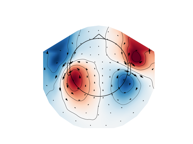
Plot magnetometer data as an arrowmap along with the topoplot at the time of the maximum sensor space activity:

max_time_idx = np.abs(evoked_mag.data).mean(axis=0).argmax()
plot_arrowmap(evoked_mag.data[:, max_time_idx], evoked_mag.info)

# Since planar gradiometers takes gradients along latitude and longitude,
# they need to be projected to the flatten manifold span by magnetometer
# or radial gradiometers before taking the gradients in the 2D Cartesian
# coordinate system for visualization on the 2D topoplot. You can use the
# ``info_from`` and ``info_to`` parameters to interpolate from
# gradiometer data to magnetometer data.

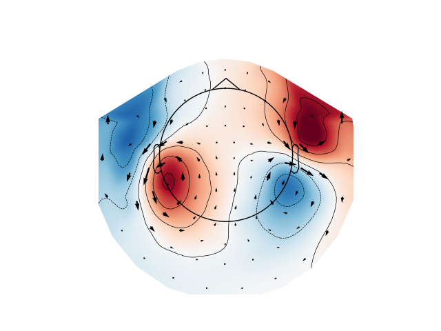
Plot gradiometer data as an arrowmap along with the topoplot at the time of the maximum sensor space activity:

plot_arrowmap(evoked_grad.data[:, max_time_idx], info_from=evoked_grad.info,
              info_to=evoked_mag.info)

Out:

Computing dot products for 203 MEG channels...
Computing cross products for 203 → 102 MEG channels...
Preparing the mapping matrix...
Truncating at 79/203 components to omit less than 0.0001 (9.2e-05)

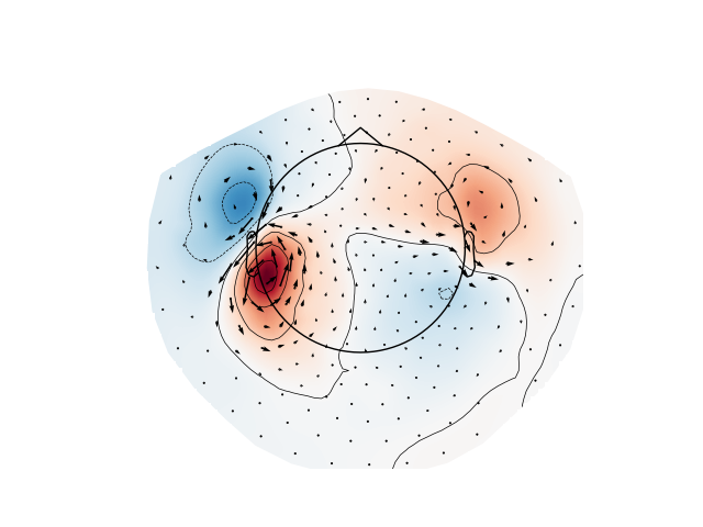
Since Vectorview 102 system perform sparse spatial sampling of the magnetic field, data from the Vectorview (info_from) can be projected to the high density CTF 272 system (info_to) for visualization

Plot gradiometer data as an arrowmap along with the topoplot at the time of the maximum sensor space activity:

path = bst_raw.data_path()
raw_fname = path + ('/MEG/bst_raw/'
                    'subj001_somatosensory_20111109_01_AUX-f.ds')
raw_ctf = mne.io.read_raw_ctf(raw_fname)
raw_ctf_info = mne.pick_info(
    raw_ctf.info, mne.pick_types(raw_ctf.info, meg=True, ref_meg=False))
plot_arrowmap(evoked_grad.data[:, max_time_idx], info_from=evoked_grad.info,
              info_to=raw_ctf_info, scale=6e-10)

Out:

ds directory : /home/circleci/mne_data/MNE-brainstorm-data/bst_raw/MEG/bst_raw/subj001_somatosensory_20111109_01_AUX-f.ds
    res4 data read.
    hc data read.
    Separate EEG position data file not present.
    Quaternion matching (desired vs. transformed):
       0.84   69.49    0.00 mm <->    0.84   69.49   -0.00 mm (orig :  -44.30   51.45 -252.43 mm) diff =    0.000 mm
      -0.84  -69.49    0.00 mm <->   -0.84  -69.49   -0.00 mm (orig :   46.28  -53.58 -243.47 mm) diff =    0.000 mm
      86.41    0.00    0.00 mm <->   86.41    0.00    0.00 mm (orig :   63.60   55.82 -230.26 mm) diff =    0.000 mm
    Coordinate transformations established.
    Reading digitizer points from ['/home/circleci/mne_data/MNE-brainstorm-data/bst_raw/MEG/bst_raw/subj001_somatosensory_20111109_01_AUX-f.ds/subj00111092011.pos']...
    Polhemus data for 3 HPI coils added
    Device coordinate locations for 3 HPI coils added
Picked positions of 2 EEG channels from channel info
    2 EEG locations added to Polhemus data.
    Measurement info composed.
Finding samples for /home/circleci/mne_data/MNE-brainstorm-data/bst_raw/MEG/bst_raw/subj001_somatosensory_20111109_01_AUX-f.ds/subj001_somatosensory_20111109_01_AUX-f.meg4:
    System clock channel is available, checking which samples are valid.
    240 x 1800 = 432000 samples from 302 chs
Current compensation grade : 3
Removing 5 compensators from info because not all compensation channels were picked.
    Computing dot products for 203 MEG channels...
    Computing cross products for 203 → 272 MEG channels...
    Preparing the mapping matrix...
    Truncating at 79/203 components to omit less than 0.0001 (9.2e-05)

Estimated memory usage: 8 MB