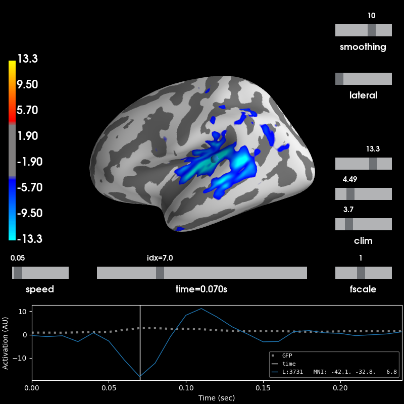
Cross-hemisphere comparison¶

This example illustrates how to visualize the difference between activity in the left and the right hemisphere. The data from the right hemisphere is mapped to the left hemisphere, and then the difference is plotted. For more information see mne.compute_source_morph().

Out:

Using control points [ 3.70314401  4.48867635 13.29875944]

# Author: Christian Brodbeck <christianbrodbeck@nyu.edu>
#
# License: BSD (3-clause)

import mne

data_dir = mne.datasets.sample.data_path()
subjects_dir = data_dir + '/subjects'
stc_path = data_dir + '/MEG/sample/sample_audvis-meg-eeg'
stc = mne.read_source_estimate(stc_path, 'sample')

# First, morph the data to fsaverage_sym, for which we have left_right
# registrations:
stc = mne.compute_source_morph(stc, 'sample', 'fsaverage_sym', smooth=5,
                               warn=False,
                               subjects_dir=subjects_dir).apply(stc)

# Compute a morph-matrix mapping the right to the left hemisphere,
# and vice-versa.
morph = mne.compute_source_morph(stc, 'fsaverage_sym', 'fsaverage_sym',
                                 spacing=stc.vertices, warn=False,
                                 subjects_dir=subjects_dir, xhemi=True,
                                 verbose='error')  # creating morph map
stc_xhemi = morph.apply(stc)

# Now we can subtract them and plot the result:
diff = stc - stc_xhemi

diff.plot(hemi='lh', subjects_dir=subjects_dir, initial_time=0.07,
          size=(800, 600))