Note
Click here to download the full example code
Background on Independent Component Analysis (ICA)
Many M/EEG signals including biological artifacts reflect non-Gaussian
processes. Therefore PCA-based artifact rejection will likely perform worse at
separating the signal from noise sources.
MNE-Python supports identifying artifacts and latent components using temporal ICA.
MNE-Python implements the mne.preprocessing.ICA class that facilitates applying ICA
to MEG and EEG data. Here we discuss some
basics of ICA.
Concepts
ICA finds directions in the feature space corresponding to projections with high non-Gaussianity.
not necessarily orthogonal in the original feature space, but orthogonal in the whitened feature space.
In contrast, PCA finds orthogonal directions in the raw feature space that correspond to directions accounting for maximum variance.
or differently, if data only reflect Gaussian processes ICA and PCA are equivalent.
Example: Imagine 3 instruments playing simultaneously and 3 microphones recording mixed signals. ICA can be used to recover the sources ie. what is played by each instrument.
ICA employs a very simple model: \(X = AS\) where \(X\) is our observations, \(A\) is the mixing matrix and \(S\) is the vector of independent (latent) sources.
The challenge is to recover \(A\) and \(S\) from \(X\).
First generate simulated data
import numpy as np
import matplotlib.pyplot as plt
from scipy import signal

from sklearn.decomposition import FastICA, PCA

np.random.seed(0)  # set seed for reproducible results
n_samples = 2000
time = np.linspace(0, 8, n_samples)

s1 = np.sin(2 * time)  # Signal 1 : sinusoidal signal
s2 = np.sign(np.sin(3 * time))  # Signal 2 : square signal
s3 = signal.sawtooth(2 * np.pi * time)  # Signal 3: sawtooth signal

S = np.c_[s1, s2, s3]
S += 0.2 * np.random.normal(size=S.shape)  # Add noise

S /= S.std(axis=0)  # Standardize data
# Mix data
A = np.array([[1, 1, 1], [0.5, 2, 1.0], [1.5, 1.0, 2.0]])  # Mixing matrix
X = np.dot(S, A.T)  # Generate observations
Now try to recover the sources
# compute ICA
ica = FastICA(n_components=3)
S_ = ica.fit_transform(X)  # Get the estimated sources
A_ = ica.mixing_  # Get estimated mixing matrix

# compute PCA
pca = PCA(n_components=3)
H = pca.fit_transform(X)  # estimate PCA sources

plt.figure(figsize=(9, 6))

models = [X, S, S_, H]
names = ['Observations (mixed signal)',
         'True Sources',
         'ICA estimated sources',
         'PCA estimated sources']
colors = ['red', 'steelblue', 'orange']

for ii, (model, name) in enumerate(zip(models, names), 1):
    plt.subplot(4, 1, ii)
    plt.title(name)
    for sig, color in zip(model.T, colors):
        plt.plot(sig, color=color)

plt.tight_layout()
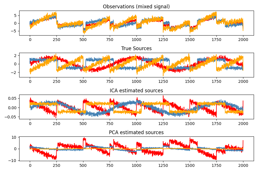
\(\rightarrow\) PCA fails at recovering our “instruments” since the related signals reflect non-Gaussian processes.
Total running time of the script: ( 0 minutes 3.492 seconds)
Estimated memory usage: 8 MB