Note
Click here to download the full example code
Exporting Epochs to Pandas DataFrames
This tutorial shows how to export the data in Epochs objects to a
Pandas DataFrame, and applies a typical Pandas
split-apply-combine workflow to examine the
latencies of the response maxima across epochs and conditions.
Page contents
We’ll use the Sample dataset, but load a version of the raw file that has already been filtered and downsampled, and has an average reference applied to its EEG channels. As usual we’ll start by importing the modules we need and loading the data:
import os
import seaborn as sns
import mne

sample_data_folder = mne.datasets.sample.data_path()
sample_data_raw_file = os.path.join(sample_data_folder, 'MEG', 'sample',
                                    'sample_audvis_filt-0-40_raw.fif')
raw = mne.io.read_raw_fif(sample_data_raw_file, verbose=False)
Next we’ll load a list of events from file, map them to condition names with an event dictionary, set some signal rejection thresholds (cf. Rejecting Epochs based on channel amplitude), and segment the continuous data into epochs:
sample_data_events_file = os.path.join(sample_data_folder, 'MEG', 'sample',
                                       'sample_audvis_filt-0-40_raw-eve.fif')
events = mne.read_events(sample_data_events_file)

event_dict = {'auditory/left': 1, 'auditory/right': 2, 'visual/left': 3,
              'visual/right': 4}

reject_criteria = dict(mag=3000e-15,     # 3000 fT
                       grad=3000e-13,    # 3000 fT/cm
                       eeg=100e-6,       # 100 µV
                       eog=200e-6)       # 200 µV

tmin, tmax = (-0.2, 0.5)  # epoch from 200 ms before event to 500 ms after it
baseline = (None, 0)      # baseline period from start of epoch to time=0

epochs = mne.Epochs(raw, events, event_dict, tmin, tmax, proj=True,
                    baseline=baseline, reject=reject_criteria, preload=True)
del raw
Out:
Not setting metadata
Not setting metadata
288 matching events found
Applying baseline correction (mode: mean)
Created an SSP operator (subspace dimension = 4)
4 projection items activated
Loading data for 288 events and 106 original time points ...
    Rejecting  epoch based on EEG : ['EEG 003']
    Rejecting  epoch based on EEG : ['EEG 001', 'EEG 002', 'EEG 003', 'EEG 004', 'EEG 006', 'EEG 007']
    Rejecting  epoch based on EEG : ['EEG 001', 'EEG 002', 'EEG 003', 'EEG 007']
    Rejecting  epoch based on EEG : ['EEG 001']
    Rejecting  epoch based on EEG : ['EEG 003', 'EEG 007']
    Rejecting  epoch based on EEG : ['EEG 007']
    Rejecting  epoch based on EEG : ['EEG 003', 'EEG 007']
    Rejecting  epoch based on EEG : ['EEG 007']
    Rejecting  epoch based on MAG : ['MEG 1411', 'MEG 1421', 'MEG 1441']
    Rejecting  epoch based on MAG : ['MEG 1711']
    Rejecting  epoch based on EEG : ['EEG 001', 'EEG 002', 'EEG 003', 'EEG 007']
    Rejecting  epoch based on EEG : ['EEG 007']
    Rejecting  epoch based on MAG : ['MEG 1411', 'MEG 1421']
    Rejecting  epoch based on MAG : ['MEG 1711']
    Rejecting  epoch based on EOG : ['EOG 061']
    Rejecting  epoch based on EEG : ['EEG 008']
    Rejecting  epoch based on EEG : ['EEG 008']
    Rejecting  epoch based on EOG : ['EOG 061']
    Rejecting  epoch based on EEG : ['EEG 007', 'EEG 008']
    Rejecting  epoch based on EEG : ['EEG 001', 'EEG 002', 'EEG 003', 'EEG 007']
    Rejecting  epoch based on EEG : ['EEG 001', 'EEG 003', 'EEG 007']
    Rejecting  epoch based on MAG : ['MEG 1411', 'MEG 1421']
    Rejecting  epoch based on MAG : ['MEG 1411']
    Rejecting  epoch based on EEG : ['EEG 001', 'EEG 002', 'EEG 003', 'EEG 007']
    Rejecting  epoch based on EEG : ['EEG 001', 'EEG 002', 'EEG 003', 'EEG 007']
    Rejecting  epoch based on EEG : ['EEG 007']
    Rejecting  epoch based on EEG : ['EEG 003', 'EEG 007']
    Rejecting  epoch based on EEG : ['EEG 003', 'EEG 007']
    Rejecting  epoch based on EEG : ['EEG 007']
    Rejecting  epoch based on MAG : ['MEG 1331', 'MEG 1421']
    Rejecting  epoch based on EEG : ['EEG 007']
    Rejecting  epoch based on EOG : ['EOG 061']
    Rejecting  epoch based on EEG : ['EEG 001', 'EEG 002', 'EEG 003', 'EEG 007']
    Rejecting  epoch based on EEG : ['EEG 001', 'EEG 002', 'EEG 003', 'EEG 007']
    Rejecting  epoch based on EEG : ['EEG 001', 'EEG 002', 'EEG 003', 'EEG 007']
35 bad epochs dropped
Converting an Epochs object to a DataFrame
Once we have our Epochs object, converting it to a
DataFrame is simple: just call epochs.to_data_frame(). Each channel’s data will be a column of the new
DataFrame, alongside three additional columns of event name,
epoch number, and sample time. Here we’ll just show the first few rows and
columns:
df = epochs.to_data_frame()
df.iloc[:5, :10]
Scaling time and channel values
By default, time values are converted from seconds to milliseconds and
then rounded to the nearest integer; if you don’t want this, you can pass
time_format=None to keep time as a float value in seconds, or
convert it to a Timedelta value via
time_format='timedelta'.
Note also that, by default, channel measurement values are scaled so that EEG
data are converted to µV, magnetometer data are converted to fT, and
gradiometer data are converted to fT/cm. These scalings can be customized
through the scalings parameter, or suppressed by passing
scalings=dict(eeg=1, mag=1, grad=1).
df = epochs.to_data_frame(time_format=None,
                          scalings=dict(eeg=1, mag=1, grad=1))
df.iloc[:5, :10]
Notice that the time values are no longer integers, and the channel values have changed by several orders of magnitude compared to the earlier DataFrame.
Setting the index
It is also possible to move one or more of the indicator columns (event name,
epoch number, and sample time) into the index, by
passing a string or list of strings as the index parameter. We’ll also
demonstrate here the effect of time_format='timedelta', yielding
Timedelta values in the “time” column.
df = epochs.to_data_frame(index=['condition', 'epoch'],
                          time_format='timedelta')
df.iloc[:5, :10]
Wide- versus long-format DataFrames
Another parameter, long_format, determines whether each channel’s data is
in a separate column of the DataFrame
(long_format=False), or whether the measured values are pivoted into a
single 'value' column with an extra indicator column for the channel name
(long_format=True). Passing long_format=True will also create an
extra column ch_type indicating the channel type.
long_df = epochs.to_data_frame(time_format=None, index='condition',
                               long_format=True)
long_df.head()
Out:
Converting "epoch" to "category"...
Converting "channel" to "category"...
Converting "ch_type" to "category"...
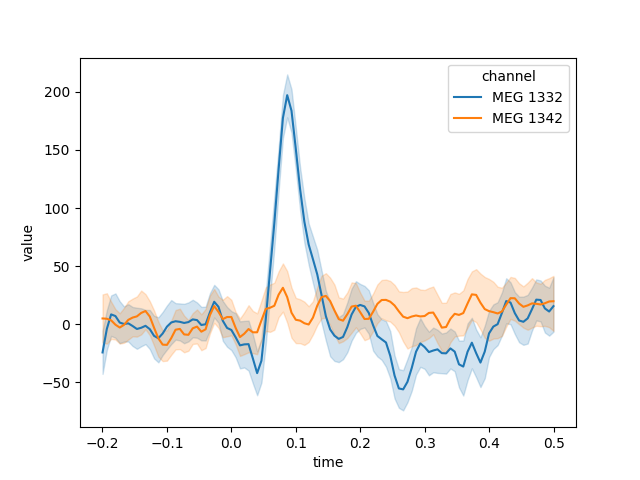
Generating the DataFrame in long format can be helpful when
using other Python modules for subsequent analysis or plotting. For example,
here we’ll take data from the “auditory/left” condition, pick a couple MEG
channels, and use seaborn.lineplot() to automatically plot the mean and
confidence band for each channel, with confidence computed across the epochs
in the chosen condition:
channels = ['MEG 1332', 'MEG 1342']
data = long_df.loc['auditory/left'].query('channel in @channels')
# convert channel column (CategoryDtype → string; for a nicer-looking legend)
data['channel'] = data['channel'].astype(str)
sns.lineplot(x='time', y='value', hue='channel', data=data)
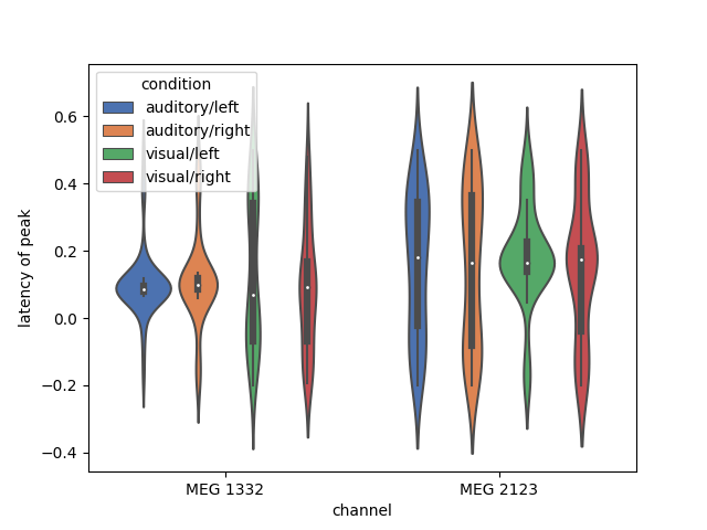
We can also now use all the power of Pandas for grouping and transforming our
data. Here, we find the latency of peak activation of 2 gradiometers (one
near auditory cortex and one near visual cortex), and plot the distribution
of the timing of the peak in each channel as a violinplot():
df = epochs.to_data_frame(time_format=None)
peak_latency = (df.filter(regex=r'condition|epoch|MEG 1332|MEG 2123')
                .groupby(['condition', 'epoch'])
                .aggregate(lambda x: df['time'].iloc[x.idxmax()])
                .reset_index()
                .melt(id_vars=['condition', 'epoch'],
                      var_name='channel',
                      value_name='latency of peak')
                )

ax = sns.violinplot(x='channel', y='latency of peak', hue='condition',
                    data=peak_latency, palette='deep', saturation=1)
Total running time of the script: ( 0 minutes 15.056 seconds)
Estimated memory usage: 847 MB