Estimation of the slope and intercept of the Power Spectral Density¶

This example aims at showing how the utility function power_spectrum and the feature function mne_features.univariate.compute_spect_slope() can be used to estimate the slope and the intercept of the Power Spectral Density (PSD, computed - by default - using Welch method).

The code for this example is based on the method proposed in:

Jean-Baptiste SCHIRATTI, Jean-Eudes LE DOUGET, Michel LE VAN QUYEN, Slim ESSID, Alexandre GRAMFORT, “An ensemble learning approach to detect epileptic seizures from long intracranial EEG recordings” Proc. IEEE ICASSP Conf. 2018

Note

This example is for illustration purposes, as other methods may lead to more robust/reliable estimation of the slope and intercept of the PSD.

# Author: Jean-Baptiste Schiratti <jean.baptiste.schiratti@gmail.com>
#         Alexandre Gramfort <alexandre.gramfort@inria.fr>
# License: BSD 3 clause

import matplotlib.pyplot as plt
import mne
import numpy as np
from mne.datasets import sample

from mne_features.univariate import compute_spect_slope
from mne_features.utils import power_spectrum

print(__doc__)

Let us import the data using MNE-Python and epoch it:

data_path = sample.data_path()
raw_fname = data_path + '/MEG/sample/sample_audvis_filt-0-40_raw.fif'
event_fname = data_path + '/MEG/sample/sample_audvis_filt-0-40_raw-eve.fif'
tmin, tmax = -0.2, 0.5
event_id = dict(aud_l=1, vis_l=3)

# Setup for reading the raw data
raw = mne.io.read_raw_fif(raw_fname, preload=True)
raw.filter(.5, None, fir_design='firwin')

Measurement date	December 03, 2002 19:01:10 GMT
Experimenter	Unknown
Participant	Unknown
Digitized points	146 points
Good channels	204 Gradiometers, 102 Magnetometers, 9 Stimulus, 60 EEG, 1 EOG
Bad channels	MEG 2443, EEG 053
EOG channels	EOG 061
ECG channels	Not available
Sampling frequency	150.15 Hz
Highpass	0.50 Hz
Lowpass	40.00 Hz
Projections	PCA-v1: off PCA-v2: off PCA-v3: off Average EEG reference: off
Filenames	sample_audvis_filt-0-40_raw.fif
Duration	00:04:37 (HH:MM:SS)

Estimate the slope (and the intercept) of the PSD. We use here a single MEG channel during the full recording to estimate the slope and the intercept.

data, _ = raw[1, :2048]
sfreq = raw.info['sfreq']

# Compute the (one-sided) PSD using Welch method. The ``mask`` variable allows
# to select only the part of the PSD which corresponds to frequencies between
# 0.1Hz and 40Hz (the data used in this example is already low-pass filtered
# at 40Hz).
psd, freqs = power_spectrum(sfreq, data)
mask = np.logical_and(1 <= freqs, freqs <= 40)
psd, freqs = psd[0, mask], freqs[mask]

# Estimate the slope (and the intercept) of the PSD. The function
# :func:`compute_spect_slope` assumes that the PSD of the signal is of the
# form: ``psd[f] = b / (f ** a)``. The coefficients a and b are respectively
# called *slope* and *intercept* of the Power Spectral Density. The values of
# the variables ``slope`` and ``intercept`` differ from the values returned
# by ``compute_spect_slope`` because, in the feature function, the linear
# regression fit is done in the log10-log10 scale.
intercept, slope, _, _ = compute_spect_slope(sfreq, data, fmin=1., fmax=40.)
print('The estimated slope is a = %1.2f and the estimated intercept is '
      'b = %1.3e' % (slope, intercept))

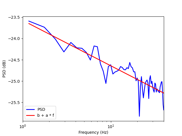
# Plot the PSD together with the ``b + a * f`` straight line (estimated decay
# of the PSD with frequency in the log10-log10 scale).
plt.figure()
plt.semilogx(freqs, np.log10(psd), '-b', lw=2, label='PSD')
plt.semilogx(freqs, intercept + slope * np.log10(freqs),
             '-r', lw=2, label='b + a * f')
plt.xlabel('Frequency (Hz)')
plt.ylabel('PSD (dB)')
plt.xlim([1, 40])
plt.legend(loc='lower left')
plt.show()

Out:

The estimated slope is a = -1.07 and the estimated intercept is b = -2.357e+01

Total running time of the script: ( 0 minutes 0.839 seconds)

Gallery generated by Sphinx-Gallery