Apply reference channel correction
Apply reference channels and see what happens.
# Author: Denis A. Enegemann
# License: BSD 3 clause

# import os
import os.path as op

import numpy as np
import matplotlib.pyplot as plt
from scipy.signal import welch

import mne
import hcp
from hcp.preprocessing import apply_ref_correction
We first set parameters
storage_dir = op.join(op.expanduser('~'), 'mne-hcp-data')
hcp_path = op.join(storage_dir, 'HCP')
subject = '105923'
data_type = 'rest'
run_index = 0
Then we define a spectral plotter for convenience
Now we read in the data
Then we plot the power spectrum of the MEG and reference channels, apply the reference correction and add the resulting cleaned MEG channels to our comparison.
raw = hcp.read_raw(subject=subject, hcp_path=hcp_path,
                   run_index=run_index, data_type=data_type)
raw.load_data()

# get meg and ref channels
meg_picks = mne.pick_types(raw.info, meg=True, ref_meg=False)
ref_picks = mne.pick_types(raw.info, ref_meg=True, meg=False)


# put single channel aside for comparison later
chan1 = raw[meg_picks[0]][0]

# add some plotting parameter
decim_fit = 100  # we lean a purely spatial model, we don't need all samples
decim_show = 10  # we can make plotting faster
n_fft = 2 ** 15  # let's use long windows to see low frequencies

# we put aside the time series for later plotting
x_meg = raw[meg_picks][0][:, ::decim_show].mean(0)
x_meg_ref = raw[ref_picks][0][:, ::decim_show].mean(0)
Now we apply the ref correction (in place).
apply_ref_correction(raw)
That was the easiest part! Let’s now plot everything.
plt.figure(figsize=(9, 6))
plot_psd(x_meg, Fs=raw.info['sfreq'], NFFT=n_fft, label='MEG', color='black')
plot_psd(x_meg_ref, Fs=raw.info['sfreq'], NFFT=n_fft, label='MEG-REF',
         color='red')
plot_psd(raw[meg_picks][0][:, ::decim_show].mean(0), Fs=raw.info['sfreq'],
         NFFT=n_fft, label='MEG-corrected', color='orange')

plt.legend()
plt.xticks(np.log10([0.1, 1, 10, 100]), [0.1, 1, 10, 100])
plt.xlim(np.log10([0.1, 300]))
plt.xlabel('log10(frequency) [Hz]')
plt.ylabel('Power Spectral Density [dB]')
plt.grid()
plt.show()
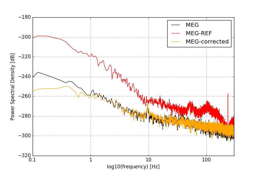
We can see that the ref correction removes low frequencies which is expected
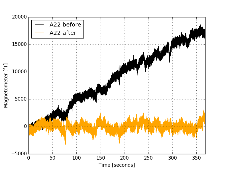
By comparing single channel time series we can also see the detrending effect
chan1c = raw[meg_picks[0]][0]
ch_name = raw.ch_names[meg_picks[0]]

plt.figure()
plt.plot(raw.times, chan1.ravel() * 1e15, label='%s before' % ch_name,
         color='black')
plt.plot(raw.times, chan1c.ravel() * 1e15, label='%s after' % ch_name,
         color='orange')
plt.xlim(raw.times[[0, -1]])
plt.legend(loc='upper left')
plt.ylabel('Magnetometer [fT]')
plt.xlabel('Time [seconds]')
plt.grid()
plt.show()
Total running time of the script: ( 0 minutes 16.880 seconds)