Note
Click here to download the full example code
Compute coherence in source space using a MNE inverse solution
This example computes the coherence between a seed in the left auditory cortex and the rest of the brain based on single-trial MNE-dSPM inverse solutions.
# Author: Martin Luessi <mluessi@nmr.mgh.harvard.edu>
#
# License: BSD (3-clause)

import numpy as np

import mne
from mne.datasets import sample
from mne.minimum_norm import (apply_inverse, apply_inverse_epochs,
                              read_inverse_operator)
from mne.connectivity import seed_target_indices, spectral_connectivity

print(__doc__)
Read the data
First we’ll read in the sample MEG data that we’ll use for computing coherence between channels. We’ll convert this into epochs in order to compute the event-related coherence.
data_path = sample.data_path()
subjects_dir = data_path + '/subjects'
fname_inv = data_path + '/MEG/sample/sample_audvis-meg-oct-6-meg-inv.fif'
fname_raw = data_path + '/MEG/sample/sample_audvis_filt-0-40_raw.fif'
fname_event = data_path + '/MEG/sample/sample_audvis_filt-0-40_raw-eve.fif'
label_name_lh = 'Aud-lh'
fname_label_lh = data_path + '/MEG/sample/labels/%s.label' % label_name_lh

event_id, tmin, tmax = 1, -0.2, 0.5
method = "dSPM"  # use dSPM method (could also be MNE or sLORETA)

# Load data.
inverse_operator = read_inverse_operator(fname_inv)
label_lh = mne.read_label(fname_label_lh)
raw = mne.io.read_raw_fif(fname_raw)
events = mne.read_events(fname_event)

# Add a bad channel.
raw.info['bads'] += ['MEG 2443']

# pick MEG channels.
picks = mne.pick_types(raw.info, meg=True, eeg=False, stim=False, eog=True,
                       exclude='bads')

# Read epochs.
epochs = mne.Epochs(raw, events, event_id, tmin, tmax, picks=picks,
                    baseline=(None, 0),
                    reject=dict(mag=4e-12, grad=4000e-13, eog=150e-6))
Out:
Reading inverse operator decomposition from /home/circleci/mne_data/MNE-sample-data/MEG/sample/sample_audvis-meg-oct-6-meg-inv.fif...
    Reading inverse operator info...
    [done]
    Reading inverse operator decomposition...
    [done]
    305 x 305 full covariance (kind = 1) found.
    Read a total of 4 projection items:
        PCA-v1 (1 x 10²) active
        PCA-v2 (1 x 10²) active
        PCA-v3 (1 x 10²) active
        Average EEG reference (1 x 60) active
    Noise covariance matrix read.
    22494 x 22494 diagonal covariance (kind = 2) found.
    Source covariance matrix read.
    22494 x 22494 diagonal covariance (kind = 6) found.
    Orientation priors read.
    22494 x 22494 diagonal covariance (kind = 5) found.
    Depth priors read.
    Did not find the desired covariance matrix (kind = 3)
    Reading a source space...
    Computing patch statistics...
    Patch information added...
    Distance information added...
    [done]
    Reading a source space...
    Computing patch statistics...
    Patch information added...
    Distance information added...
    [done]
    2 source spaces read
    Read a total of 4 projection items:
        PCA-v1 (1 x 10²) active
        PCA-v2 (1 x 10²) active
        PCA-v3 (1 x 10²) active
        Average EEG reference (1 x 60) active
    Source spaces transformed to the inverse solution coordinate frame
Opening raw data file /home/circleci/mne_data/MNE-sample-data/MEG/sample/sample_audvis_filt-0-40_raw.fif...
    Read a total of 4 projection items:
        PCA-v1 (1 x 10²)  idle
        PCA-v2 (1 x 10²)  idle
        PCA-v3 (1 x 10²)  idle
        Average EEG reference (1 x 60)  idle
    Range : 6450 ... 48149 =     42.956 ...   320.665 secs
Ready.
Not setting metadata
Not setting metadata
72 matching events found
Applying baseline correction (mode: mean)
Created an SSP operator (subspace dimension = 3)
4 projection items activated
Choose channels for coherence estimation
Next we’ll calculate our channel sources. Then we’ll find the most active vertex in the left auditory cortex, which we will later use as seed for the connectivity computation.
snr = 3.0
lambda2 = 1.0 / snr ** 2
evoked = epochs.average()
stc = apply_inverse(evoked, inverse_operator, lambda2, method,
                    pick_ori="normal")

# Restrict the source estimate to the label in the left auditory cortex.
stc_label = stc.in_label(label_lh)

# Find number and index of vertex with most power.
src_pow = np.sum(stc_label.data ** 2, axis=1)
seed_vertno = stc_label.vertices[0][np.argmax(src_pow)]
seed_idx = np.searchsorted(stc.vertices[0], seed_vertno)  # index in orig stc

# Generate index parameter for seed-based connectivity analysis.
n_sources = stc.data.shape[0]
indices = seed_target_indices([seed_idx], np.arange(n_sources))
Out:
    Rejecting  epoch based on EOG : ['EOG 061']
    Rejecting  epoch based on EOG : ['EOG 061']
    Rejecting  epoch based on EOG : ['EOG 061']
    Rejecting  epoch based on EOG : ['EOG 061']
    Rejecting  epoch based on EOG : ['EOG 061']
    Rejecting  epoch based on MAG : ['MEG 1711']
    Rejecting  epoch based on EOG : ['EOG 061']
    Rejecting  epoch based on EOG : ['EOG 061']
    Rejecting  epoch based on EOG : ['EOG 061']
    Rejecting  epoch based on EOG : ['EOG 061']
    Rejecting  epoch based on EOG : ['EOG 061']
    Rejecting  epoch based on EOG : ['EOG 061']
    Rejecting  epoch based on EOG : ['EOG 061']
    Rejecting  epoch based on EOG : ['EOG 061']
    Rejecting  epoch based on EOG : ['EOG 061']
    Rejecting  epoch based on EOG : ['EOG 061']
    Rejecting  epoch based on EOG : ['EOG 061']
Removing projector <Projection | Average EEG reference, active : True, n_channels : 60>
Preparing the inverse operator for use...
    Scaled noise and source covariance from nave = 1 to nave = 55
    Created the regularized inverter
    Created an SSP operator (subspace dimension = 3)
    Created the whitener using a noise covariance matrix with rank 302 (3 small eigenvalues omitted)
    Computing noise-normalization factors (dSPM)...
[done]
Applying inverse operator to "1"...
    Picked 305 channels from the data
    Computing inverse...
    Eigenleads need to be weighted ...
    Computing residual...
    Explained  59.3% variance
    dSPM...
[done]
Compute the inverse solution for each epoch. By using “return_generator=True” stcs will be a generator object instead of a list. This allows us so to compute the coherence without having to keep all source estimates in memory.
snr = 1.0  # use lower SNR for single epochs
lambda2 = 1.0 / snr ** 2
stcs = apply_inverse_epochs(epochs, inverse_operator, lambda2, method,
                            pick_ori="normal", return_generator=True)
Compute the coherence between sources
Now we are ready to compute the coherence in the alpha and beta band. fmin and fmax specify the lower and upper freq. for each band, respectively.
To speed things up, we use 2 parallel jobs and use mode=’fourier’, which uses a FFT with a Hanning window to compute the spectra (instead of a multitaper estimation, which has a lower variance but is slower). By using faverage=True, we directly average the coherence in the alpha and beta band, i.e., we will only get 2 frequency bins.
fmin = (8., 13.)
fmax = (13., 30.)
sfreq = raw.info['sfreq']  # the sampling frequency

coh, freqs, times, n_epochs, n_tapers = spectral_connectivity(
    stcs, method='coh', mode='fourier', indices=indices,
    sfreq=sfreq, fmin=fmin, fmax=fmax, faverage=True, n_jobs=1)

print('Frequencies in Hz over which coherence was averaged for alpha: ')
print(freqs[0])
print('Frequencies in Hz over which coherence was averaged for beta: ')
print(freqs[1])
Out:
Connectivity computation...
Preparing the inverse operator for use...
    Scaled noise and source covariance from nave = 1 to nave = 1
    Created the regularized inverter
    Created an SSP operator (subspace dimension = 3)
    Created the whitener using a noise covariance matrix with rank 302 (3 small eigenvalues omitted)
    Computing noise-normalization factors (dSPM)...
[done]
Picked 305 channels from the data
Computing inverse...
    Eigenleads need to be weighted ...
Processing epoch : 1 / 72 (at most)
    computing connectivity for 7498 connections
    using t=-0.200s..0.499s for estimation (106 points)
    computing connectivity for the bands:
     band 1: 8.5Hz..12.7Hz (4 points)
     band 2: 14.2Hz..29.7Hz (12 points)
    connectivity scores will be averaged for each band
    using FFT with a Hanning window to estimate spectra
    the following metrics will be computed: Coherence
    computing connectivity for epoch 1
Processing epoch : 2 / 72 (at most)
    computing connectivity for epoch 2
Processing epoch : 3 / 72 (at most)
    computing connectivity for epoch 3
Processing epoch : 4 / 72 (at most)
    computing connectivity for epoch 4
Processing epoch : 5 / 72 (at most)
    computing connectivity for epoch 5
Processing epoch : 6 / 72 (at most)
    computing connectivity for epoch 6
Processing epoch : 7 / 72 (at most)
    computing connectivity for epoch 7
Processing epoch : 8 / 72 (at most)
    computing connectivity for epoch 8
Processing epoch : 9 / 72 (at most)
    computing connectivity for epoch 9
Processing epoch : 10 / 72 (at most)
    computing connectivity for epoch 10
    Rejecting  epoch based on EOG : ['EOG 061']
Processing epoch : 11 / 72 (at most)
    computing connectivity for epoch 11
Processing epoch : 12 / 72 (at most)
    computing connectivity for epoch 12
Processing epoch : 13 / 72 (at most)
    computing connectivity for epoch 13
    Rejecting  epoch based on EOG : ['EOG 061']
    Rejecting  epoch based on EOG : ['EOG 061']
Processing epoch : 14 / 72 (at most)
    computing connectivity for epoch 14
Processing epoch : 15 / 72 (at most)
    computing connectivity for epoch 15
Processing epoch : 16 / 72 (at most)
    computing connectivity for epoch 16
Processing epoch : 17 / 72 (at most)
    computing connectivity for epoch 17
    Rejecting  epoch based on EOG : ['EOG 061']
Processing epoch : 18 / 72 (at most)
    computing connectivity for epoch 18
Processing epoch : 19 / 72 (at most)
    computing connectivity for epoch 19
Processing epoch : 20 / 72 (at most)
    computing connectivity for epoch 20
    Rejecting  epoch based on EOG : ['EOG 061']
Processing epoch : 21 / 72 (at most)
    computing connectivity for epoch 21
Processing epoch : 22 / 72 (at most)
    computing connectivity for epoch 22
Processing epoch : 23 / 72 (at most)
    computing connectivity for epoch 23
    Rejecting  epoch based on MAG : ['MEG 1711']
Processing epoch : 24 / 72 (at most)
    computing connectivity for epoch 24
Processing epoch : 25 / 72 (at most)
    computing connectivity for epoch 25
Processing epoch : 26 / 72 (at most)
    computing connectivity for epoch 26
Processing epoch : 27 / 72 (at most)
    computing connectivity for epoch 27
Processing epoch : 28 / 72 (at most)
    computing connectivity for epoch 28
    Rejecting  epoch based on EOG : ['EOG 061']
Processing epoch : 29 / 72 (at most)
    computing connectivity for epoch 29
Processing epoch : 30 / 72 (at most)
    computing connectivity for epoch 30
Processing epoch : 31 / 72 (at most)
    computing connectivity for epoch 31
    Rejecting  epoch based on EOG : ['EOG 061']
Processing epoch : 32 / 72 (at most)
    computing connectivity for epoch 32
Processing epoch : 33 / 72 (at most)
    computing connectivity for epoch 33
    Rejecting  epoch based on EOG : ['EOG 061']
Processing epoch : 34 / 72 (at most)
    computing connectivity for epoch 34
Processing epoch : 35 / 72 (at most)
    computing connectivity for epoch 35
    Rejecting  epoch based on EOG : ['EOG 061']
    Rejecting  epoch based on EOG : ['EOG 061']
Processing epoch : 36 / 72 (at most)
    computing connectivity for epoch 36
    Rejecting  epoch based on EOG : ['EOG 061']
    Rejecting  epoch based on EOG : ['EOG 061']
Processing epoch : 37 / 72 (at most)
    computing connectivity for epoch 37
Processing epoch : 38 / 72 (at most)
    computing connectivity for epoch 38
Processing epoch : 39 / 72 (at most)
    computing connectivity for epoch 39
Processing epoch : 40 / 72 (at most)
    computing connectivity for epoch 40
Processing epoch : 41 / 72 (at most)
    computing connectivity for epoch 41
Processing epoch : 42 / 72 (at most)
    computing connectivity for epoch 42
Processing epoch : 43 / 72 (at most)
    computing connectivity for epoch 43
Processing epoch : 44 / 72 (at most)
    computing connectivity for epoch 44
    Rejecting  epoch based on EOG : ['EOG 061']
Processing epoch : 45 / 72 (at most)
    computing connectivity for epoch 45
    Rejecting  epoch based on EOG : ['EOG 061']
Processing epoch : 46 / 72 (at most)
    computing connectivity for epoch 46
Processing epoch : 47 / 72 (at most)
    computing connectivity for epoch 47
Processing epoch : 48 / 72 (at most)
    computing connectivity for epoch 48
    Rejecting  epoch based on EOG : ['EOG 061']
    Rejecting  epoch based on EOG : ['EOG 061']
Processing epoch : 49 / 72 (at most)
    computing connectivity for epoch 49
Processing epoch : 50 / 72 (at most)
    computing connectivity for epoch 50
Processing epoch : 51 / 72 (at most)
    computing connectivity for epoch 51
Processing epoch : 52 / 72 (at most)
    computing connectivity for epoch 52
Processing epoch : 53 / 72 (at most)
    computing connectivity for epoch 53
Processing epoch : 54 / 72 (at most)
    computing connectivity for epoch 54
Processing epoch : 55 / 72 (at most)
    computing connectivity for epoch 55
[done]
[Connectivity computation done]
Frequencies in Hz over which coherence was averaged for alpha:
[ 8.49926873  9.91581352 11.33235831 12.74890309]
Frequencies in Hz over which coherence was averaged for beta:
[14.16544788 15.58199267 16.99853746 18.41508225 19.83162704 21.24817182
 22.66471661 24.0812614  25.49780619 26.91435098 28.33089577 29.74744055]
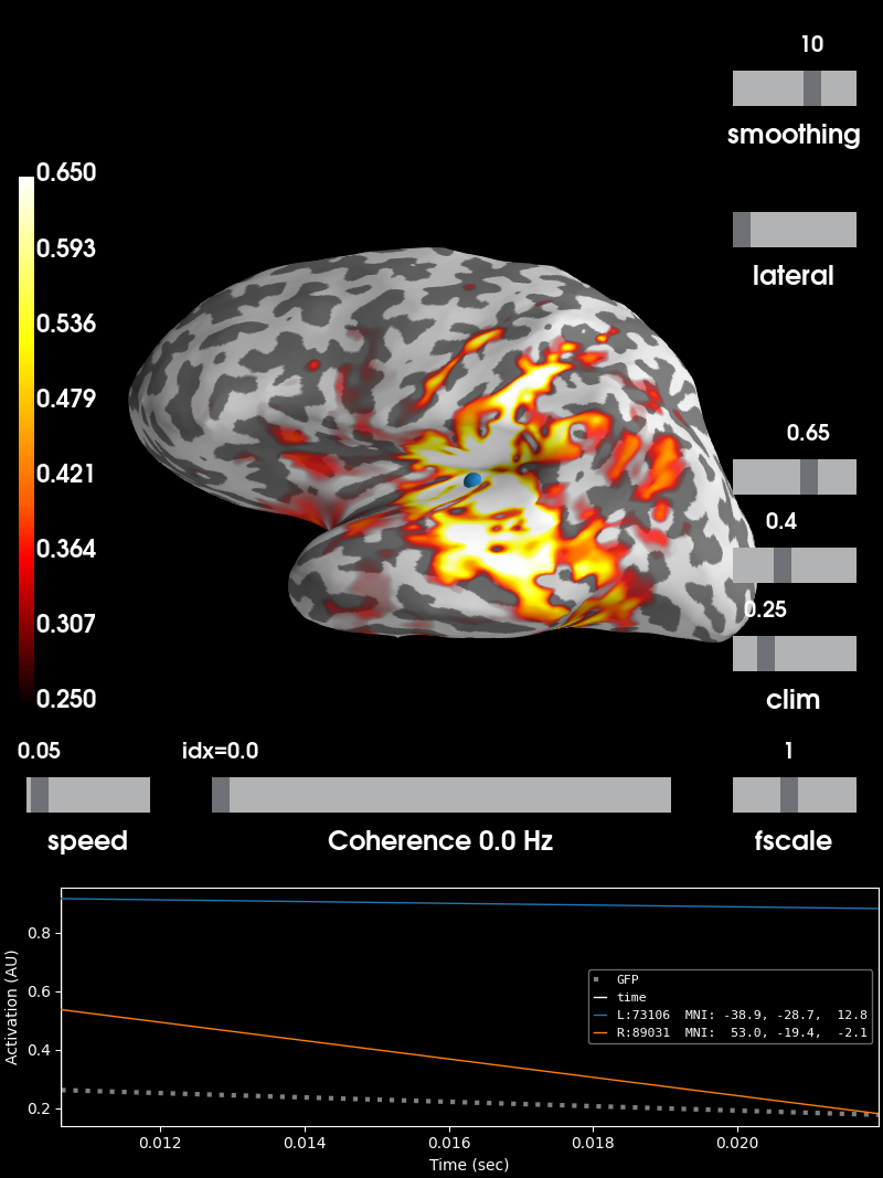
Generate coherence sources and plot
Finally, we’ll generate a SourceEstimate with the coherence. This is simple
since we used a single seed. For more than one seed we would have to choose
one of the slices within coh.
Note
We use a hack to save the frequency axis as time.
Finally, we’ll plot this source estimate on the brain.
tmin = np.mean(freqs[0])
tstep = np.mean(freqs[1]) - tmin
coh_stc = mne.SourceEstimate(coh, vertices=stc.vertices, tmin=1e-3 * tmin,
                             tstep=1e-3 * tstep, subject='sample')

# Now we can visualize the coherence using the plot method.
brain = coh_stc.plot('sample', 'inflated', 'both',
                     time_label='Coherence %0.1f Hz',
                     subjects_dir=subjects_dir,
                     clim=dict(kind='value', lims=(0.25, 0.4, 0.65)))
brain.show_view('lateral')
Total running time of the script: ( 0 minutes 19.381 seconds)
Estimated memory usage: 16 MB