Note
Click here to download the full example code
Compute envelope correlations in volume source space
Compute envelope correlations of orthogonalized activity 1 2 in source space using resting state CTF data in a volume source space.
# Authors: Eric Larson <larson.eric.d@gmail.com>
#          Sheraz Khan <sheraz@khansheraz.com>
#          Denis Engemann <denis.engemann@gmail.com>
#
# License: BSD (3-clause)

import os.path as op

import mne
from mne.beamformer import make_lcmv, apply_lcmv_epochs
from mne.connectivity import envelope_correlation
from mne.preprocessing import compute_proj_ecg, compute_proj_eog

data_path = mne.datasets.brainstorm.bst_resting.data_path()
subjects_dir = op.join(data_path, 'subjects')
subject = 'bst_resting'
trans = op.join(data_path, 'MEG', 'bst_resting', 'bst_resting-trans.fif')
bem = op.join(subjects_dir, subject, 'bem', subject + '-5120-bem-sol.fif')
raw_fname = op.join(data_path, 'MEG', 'bst_resting',
                    'subj002_spontaneous_20111102_01_AUX.ds')
crop_to = 60.
Here we do some things in the name of speed, such as crop (which will hurt SNR) and downsample. Then we compute SSP projectors and apply them.
raw = mne.io.read_raw_ctf(raw_fname, verbose='error')
raw.crop(0, crop_to).pick_types(meg=True, eeg=False).load_data().resample(80)
raw.apply_gradient_compensation(3)
projs_ecg, _ = compute_proj_ecg(raw, n_grad=1, n_mag=2)
projs_eog, _ = compute_proj_eog(raw, n_grad=1, n_mag=2, ch_name='MLT31-4407')
raw.info['projs'] += projs_ecg
raw.info['projs'] += projs_eog
raw.apply_proj()
cov = mne.compute_raw_covariance(raw)  # compute before band-pass of interest
Out:
Including 0 SSP projectors from raw file
Running ECG SSP computation
Reconstructing ECG signal from Magnetometers
Setting up band-pass filter from 5 - 35 Hz

FIR filter parameters
---------------------
Designing a two-pass forward and reverse, zero-phase, non-causal bandpass filter:
- Windowed frequency-domain design (firwin2) method
- Hann window
- Lower passband edge: 5.00
- Lower transition bandwidth: 0.50 Hz (-12 dB cutoff frequency: 4.75 Hz)
- Upper passband edge: 35.00 Hz
- Upper transition bandwidth: 0.50 Hz (-12 dB cutoff frequency: 35.25 Hz)
- Filter length: 800 samples (10.000 sec)

Number of ECG events detected : 88 (average pulse 88 / min.)
Computing projector
Not setting metadata
Not setting metadata
88 matching events found
No baseline correction applied
0 projection items activated
Loading data for 88 events and 49 original time points ...
    Rejecting  epoch based on MAG : ['MLT31-4407', 'MRT31-4407']
    Rejecting  epoch based on MAG : ['MLT31-4407', 'MLT41-4407', 'MRT31-4407', 'MRT41-4407']
    Rejecting  epoch based on MAG : ['MLT31-4407', 'MLT41-4407', 'MRT31-4407', 'MRT41-4407']
4 bad epochs dropped
No gradiometers found. Forcing n_grad to 0
No EEG channels found. Forcing n_eeg to 0
Adding projection: axial--0.200-0.400-PCA-01
Adding projection: axial--0.200-0.400-PCA-02
Done.
Including 0 SSP projectors from raw file
Running EOG SSP computation
Using channel MLT31-4407 as EOG channel
EOG channel index for this subject is: [137]
Filtering the data to remove DC offset to help distinguish blinks from saccades
Setting up band-pass filter from 1 - 10 Hz

FIR filter parameters
---------------------
Designing a two-pass forward and reverse, zero-phase, non-causal bandpass filter:
- Windowed frequency-domain design (firwin2) method
- Hann window
- Lower passband edge: 1.00
- Lower transition bandwidth: 0.50 Hz (-12 dB cutoff frequency: 0.75 Hz)
- Upper passband edge: 10.00 Hz
- Upper transition bandwidth: 0.50 Hz (-12 dB cutoff frequency: 10.25 Hz)
- Filter length: 800 samples (10.000 sec)

Now detecting blinks and generating corresponding events
Found 12 significant peaks
Number of EOG events detected : 12
Computing projector
Not setting metadata
Not setting metadata
12 matching events found
No baseline correction applied
0 projection items activated
Loading data for 12 events and 33 original time points ...
    Rejecting  epoch based on MAG : ['MRT41-4407']
1 bad epochs dropped
No gradiometers found. Forcing n_grad to 0
No EEG channels found. Forcing n_eeg to 0
Adding projection: axial--0.200-0.200-PCA-01
Adding projection: axial--0.200-0.200-PCA-02
Done.
Using up to 300 segments
Number of samples used : 4800
[done]
Now we band-pass filter our data and create epochs.
raw.filter(14, 30)
events = mne.make_fixed_length_events(raw, duration=5.)
epochs = mne.Epochs(raw, events=events, tmin=0, tmax=5.,
                    baseline=None, reject=dict(mag=8e-13), preload=True)
del raw
Out:
Not setting metadata
Not setting metadata
12 matching events found
No baseline correction applied
Created an SSP operator (subspace dimension = 4)
4 projection items activated
Loading data for 12 events and 401 original time points ...
    Rejecting  epoch based on MAG : ['MRC42-4407', 'MRC54-4407', 'MRP12-4407', 'MRP22-4407', 'MRP23-4407']
2 bad epochs dropped
Compute the forward and inverse
# This source space is really far too coarse, but we do this for speed
# considerations here
pos = 15.  # 1.5 cm is very broad, done here for speed!
src = mne.setup_volume_source_space('bst_resting', pos, bem=bem,
                                    subjects_dir=subjects_dir, verbose=True)
fwd = mne.make_forward_solution(epochs.info, trans, src, bem)
data_cov = mne.compute_covariance(epochs)
filters = make_lcmv(epochs.info, fwd, data_cov, 0.05, cov,
                    pick_ori='max-power', weight_norm='nai')
del fwd
Out:
BEM              : /home/circleci/mne_data/MNE-brainstorm-data/bst_resting/subjects/bst_resting/bem/bst_resting-5120-bem-sol.fif
grid                  : 15.0 mm
mindist               : 5.0 mm
MRI volume            : /home/circleci/mne_data/MNE-brainstorm-data/bst_resting/subjects/bst_resting/mri/T1.mgz

Reading /home/circleci/mne_data/MNE-brainstorm-data/bst_resting/subjects/bst_resting/mri/T1.mgz...

Loaded inner skull from /home/circleci/mne_data/MNE-brainstorm-data/bst_resting/subjects/bst_resting/bem/bst_resting-5120-bem-sol.fif (2562 nodes)
Surface CM = (   3.1  -22.2   29.7) mm
Surface fits inside a sphere with radius  105.3 mm
Surface extent:
    x =  -71.2 ...   75.4 mm
    y = -110.1 ...   82.9 mm
    z =  -48.4 ...   98.1 mm
Grid extent:
    x =  -75.0 ...   90.0 mm
    y = -120.0 ...   90.0 mm
    z =  -60.0 ...  105.0 mm
2160 sources before omitting any.
1364 sources after omitting infeasible sources not within 0.0 - 105.3 mm.
Source spaces are in MRI coordinates.
Checking that the sources are inside the surface and at least    5.0 mm away (will take a few...)
    Skipping interior check for 150 sources that fit inside a sphere of radius   49.6 mm
    Skipping solid angle check for 761 points using Qhull
    791 source space points omitted because they are outside the inner skull surface.
    94 source space points omitted because of the    5.0-mm distance limit.
479 sources remaining after excluding the sources outside the surface and less than    5.0 mm inside.
Adjusting the neighborhood info.
Source space : MRI voxel -> MRI (surface RAS)
     0.015000  0.000000  0.000000     -75.00 mm
     0.000000  0.015000  0.000000    -120.00 mm
     0.000000  0.000000  0.015000     -60.00 mm
     0.000000  0.000000  0.000000       1.00
MRI volume : MRI voxel -> MRI (surface RAS)
    -0.001000  0.000000  0.000000     128.00 mm
     0.000000  0.000000  0.001000    -128.00 mm
     0.000000 -0.001000  0.000000     128.00 mm
     0.000000  0.000000  0.000000       1.00
MRI volume : MRI (surface RAS) -> RAS (non-zero origin)
     1.000000  0.000000  0.000000       0.00 mm
     0.000000  1.000000  0.000000       0.00 mm
     0.000000  0.000000  1.000000       0.00 mm
     0.000000  0.000000  0.000000       1.00
Setting up volume interpolation ...
    20223000/16777216 nonzero values for the whole brain
[done]
Source space          : <SourceSpaces: [<volume, shape=(12, 15, 12), n_used=479>] MRI (surface RAS) coords, subject 'bst_resting', ~64.6 MB>
MRI -> head transform : /home/circleci/mne_data/MNE-brainstorm-data/bst_resting/MEG/bst_resting/bst_resting-trans.fif
Measurement data      : instance of Info
Conductor model   : /home/circleci/mne_data/MNE-brainstorm-data/bst_resting/subjects/bst_resting/bem/bst_resting-5120-bem-sol.fif
Accurate field computations
Do computations in head coordinates
Free source orientations

Read 1 source spaces a total of 479 active source locations

Coordinate transformation: MRI (surface RAS) -> head
     0.999797 -0.005775 -0.019288       2.71 mm
     0.011390  0.952195  0.305279      16.66 mm
     0.016602 -0.305437  0.952068      28.47 mm
     0.000000  0.000000  0.000000       1.00

Read 272 MEG channels from info
Read  26 MEG compensation channels from info
99 coil definitions read
Coordinate transformation: MEG device -> head
     0.998490 -0.050225 -0.022235       1.90 mm
     0.052235  0.993447  0.101656      13.13 mm
     0.016984 -0.102664  0.994571      66.69 mm
     0.000000  0.000000  0.000000       1.00
5 compensation data sets in info
MEG coil definitions created in head coordinates.
Removing 5 compensators from info because not all compensation channels were picked.
Source spaces are now in head coordinates.

Setting up the BEM model using /home/circleci/mne_data/MNE-brainstorm-data/bst_resting/subjects/bst_resting/bem/bst_resting-5120-bem-sol.fif...

Loading surfaces...

Loading the solution matrix...

Homogeneous model surface loaded.
Loaded linear_collocation BEM solution from /home/circleci/mne_data/MNE-brainstorm-data/bst_resting/subjects/bst_resting/bem/bst_resting-5120-bem-sol.fif
Employing the head->MRI coordinate transform with the BEM model.
BEM model bst_resting-5120-bem-sol.fif is now set up

Source spaces are in head coordinates.
Checking that the sources are inside the surface (will take a few...)
    Skipping interior check for 150 sources that fit inside a sphere of radius   49.6 mm
    Skipping solid angle check for 0 points using Qhull

Setting up compensation data...
    272 out of 272 channels have the compensation set.
    Desired compensation data (3) found.
    All compensation channels found.
    Preselector created.
    Compensation data matrix created.
    Postselector created.

Composing the field computation matrix...
Composing the field computation matrix (compensation coils)...
Computing MEG at 479 source locations (free orientations)...

Finished.
Removing 5 compensators from info because not all compensation channels were picked.
Computing rank from data with rank=None
    Using tolerance 1e-09 (2.2e-16 eps * 272 dim * 1.7e+04  max singular value)
    Estimated rank (mag): 268
    MAG: rank 268 computed from 272 data channels with 4 projectors
    Created an SSP operator (subspace dimension = 4)
    Setting small MAG eigenvalues to zero (without PCA)
Reducing data rank from 272 -> 268
Estimating covariance using EMPIRICAL
Done.
Number of samples used : 4010
[done]
Removing 5 compensators from info because not all compensation channels were picked.
Removing 5 compensators from info because not all compensation channels were picked.
Computing rank from covariance with rank='info'
    MAG: rank 268 after 4 projectors applied to 272 channels
Computing rank from covariance with rank='info'
    MAG: rank 268 after 4 projectors applied to 272 channels
Making LCMV beamformer with rank {'mag': 268}
Computing inverse operator with 272 channels.
    272 out of 272 channels remain after picking
Selected 272 channels
Whitening the forward solution.
    Created an SSP operator (subspace dimension = 4)
Computing rank from covariance with rank={'mag': 268}
    Setting small MAG eigenvalues to zero (without PCA)
Creating the source covariance matrix
Adjusting source covariance matrix.
Computing beamformer filters for 479 sources
Filter computation complete
Compute label time series and do envelope correlation
epochs.apply_hilbert()  # faster to do in sensor space
stcs = apply_lcmv_epochs(epochs, filters, return_generator=True)
corr = envelope_correlation(stcs, verbose=True)
Out:
Processing epoch : 1
Processing epoch : 2
Processing epoch : 3
Processing epoch : 4
Processing epoch : 5
Processing epoch : 6
Processing epoch : 7
Processing epoch : 8
Processing epoch : 9
Processing epoch : 10
[done]
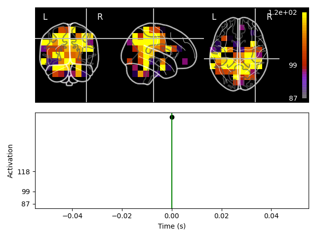
Compute the degree and plot it
degree = mne.connectivity.degree(corr, 0.15)
stc = mne.VolSourceEstimate(degree, [src[0]['vertno']], 0, 1, 'bst_resting')
brain = stc.plot(
    src, clim=dict(kind='percent', lims=[75, 85, 95]), colormap='gnuplot',
    subjects_dir=subjects_dir, mode='glass_brain')
Out:
Transforming subject RAS (non-zero origin) -> MNI Talairach
     1.029906  0.008134 -0.048341      -1.23 mm
     0.013579  0.955254  0.160974      -9.34 mm
     0.075120 -0.143988  1.092494     -28.73 mm
     0.000000  0.000000  0.000000       1.00

Showing: t = 0.000 s, (42.0, -27.7, 44.5) mm, [8, 6, 8] vox, 1520 vertex
Using control points [ 87.  99. 118.]
References
- 1
Hipp JF, Hawellek DJ, Corbetta M, Siegel M, Engel AK (2012) Large-scale cortical correlation structure of spontaneous oscillatory activity. Nature Neuroscience 15:884–890
- 2
Khan S et al. (2018). Maturation trajectories of cortical resting-state networks depend on the mediating frequency band. Neuroimage 174:57–68
Total running time of the script: ( 0 minutes 21.247 seconds)
Estimated memory usage: 599 MB