Note
Click here to download the full example code
Compute source space connectivity and visualize it using a circular graph
This example computes the all-to-all connectivity between 68 regions in source space based on dSPM inverse solutions and a FreeSurfer cortical parcellation. The connectivity is visualized using a circular graph which is ordered based on the locations of the regions in the axial plane.
# Authors: Martin Luessi <mluessi@nmr.mgh.harvard.edu>
#          Alexandre Gramfort <alexandre.gramfort@inria.fr>
#          Nicolas P. Rougier (graph code borrowed from his matplotlib gallery)
#
# License: BSD (3-clause)

import numpy as np
import matplotlib.pyplot as plt

import mne
from mne.datasets import sample
from mne.minimum_norm import apply_inverse_epochs, read_inverse_operator
from mne.connectivity import spectral_connectivity
from mne.viz import circular_layout, plot_connectivity_circle

print(__doc__)
Load our data
First we’ll load the data we’ll use in connectivity estimation. We’ll use the sample MEG data provided with MNE.
data_path = sample.data_path()
subjects_dir = data_path + '/subjects'
fname_inv = data_path + '/MEG/sample/sample_audvis-meg-oct-6-meg-inv.fif'
fname_raw = data_path + '/MEG/sample/sample_audvis_filt-0-40_raw.fif'
fname_event = data_path + '/MEG/sample/sample_audvis_filt-0-40_raw-eve.fif'

# Load data
inverse_operator = read_inverse_operator(fname_inv)
raw = mne.io.read_raw_fif(fname_raw)
events = mne.read_events(fname_event)

# Add a bad channel
raw.info['bads'] += ['MEG 2443']

# Pick MEG channels
picks = mne.pick_types(raw.info, meg=True, eeg=False, stim=False, eog=True,
                       exclude='bads')

# Define epochs for left-auditory condition
event_id, tmin, tmax = 1, -0.2, 0.5
epochs = mne.Epochs(raw, events, event_id, tmin, tmax, picks=picks,
                    baseline=(None, 0), reject=dict(mag=4e-12, grad=4000e-13,
                                                    eog=150e-6))
Out:
Reading inverse operator decomposition from /home/circleci/mne_data/MNE-sample-data/MEG/sample/sample_audvis-meg-oct-6-meg-inv.fif...
    Reading inverse operator info...
    [done]
    Reading inverse operator decomposition...
    [done]
    305 x 305 full covariance (kind = 1) found.
    Read a total of 4 projection items:
        PCA-v1 (1 x 10²) active
        PCA-v2 (1 x 10²) active
        PCA-v3 (1 x 10²) active
        Average EEG reference (1 x 60) active
    Noise covariance matrix read.
    22494 x 22494 diagonal covariance (kind = 2) found.
    Source covariance matrix read.
    22494 x 22494 diagonal covariance (kind = 6) found.
    Orientation priors read.
    22494 x 22494 diagonal covariance (kind = 5) found.
    Depth priors read.
    Did not find the desired covariance matrix (kind = 3)
    Reading a source space...
    Computing patch statistics...
    Patch information added...
    Distance information added...
    [done]
    Reading a source space...
    Computing patch statistics...
    Patch information added...
    Distance information added...
    [done]
    2 source spaces read
    Read a total of 4 projection items:
        PCA-v1 (1 x 10²) active
        PCA-v2 (1 x 10²) active
        PCA-v3 (1 x 10²) active
        Average EEG reference (1 x 60) active
    Source spaces transformed to the inverse solution coordinate frame
Opening raw data file /home/circleci/mne_data/MNE-sample-data/MEG/sample/sample_audvis_filt-0-40_raw.fif...
    Read a total of 4 projection items:
        PCA-v1 (1 x 10²)  idle
        PCA-v2 (1 x 10²)  idle
        PCA-v3 (1 x 10²)  idle
        Average EEG reference (1 x 60)  idle
    Range : 6450 ... 48149 =     42.956 ...   320.665 secs
Ready.
Not setting metadata
Not setting metadata
72 matching events found
Applying baseline correction (mode: mean)
Created an SSP operator (subspace dimension = 3)
4 projection items activated
Compute inverse solutions and their connectivity
Next, we need to compute the inverse solution for this data. This will return
the sources / source activity that we’ll use in computing connectivity. We’ll
compute the connectivity in the alpha band of these sources. We can specify
particular frequencies to include in the connectivity with the fmin and
fmax flags. Notice from the status messages how mne-python:
reads an epoch from the raw file
applies SSP and baseline correction
computes the inverse to obtain a source estimate
averages the source estimate to obtain a time series for each label
includes the label time series in the connectivity computation
moves to the next epoch.
This behaviour is because we are using generators. Since we only need to operate on the data one epoch at a time, using a generator allows us to compute connectivity in a computationally efficient manner where the amount of memory (RAM) needed is independent from the number of epochs.
# Compute inverse solution and for each epoch. By using "return_generator=True"
# stcs will be a generator object instead of a list.
snr = 1.0  # use lower SNR for single epochs
lambda2 = 1.0 / snr ** 2
method = "dSPM"  # use dSPM method (could also be MNE or sLORETA)
stcs = apply_inverse_epochs(epochs, inverse_operator, lambda2, method,
                            pick_ori="normal", return_generator=True)

# Get labels for FreeSurfer 'aparc' cortical parcellation with 34 labels/hemi
labels = mne.read_labels_from_annot('sample', parc='aparc',
                                    subjects_dir=subjects_dir)
label_colors = [label.color for label in labels]

# Average the source estimates within each label using sign-flips to reduce
# signal cancellations, also here we return a generator
src = inverse_operator['src']
label_ts = mne.extract_label_time_course(stcs, labels, src, mode='mean_flip',
                                         return_generator=True)

fmin = 8.
fmax = 13.
sfreq = raw.info['sfreq']  # the sampling frequency
con_methods = ['pli', 'wpli2_debiased', 'ciplv']
con, freqs, times, n_epochs, n_tapers = spectral_connectivity(
    label_ts, method=con_methods, mode='multitaper', sfreq=sfreq, fmin=fmin,
    fmax=fmax, faverage=True, mt_adaptive=True, n_jobs=1)

# con is a 3D array, get the connectivity for the first (and only) freq. band
# for each method
con_res = dict()
for method, c in zip(con_methods, con):
    con_res[method] = c[:, :, 0]
Out:
Reading labels from parcellation...
   read 34 labels from /home/circleci/mne_data/MNE-sample-data/subjects/sample/label/lh.aparc.annot
   read 34 labels from /home/circleci/mne_data/MNE-sample-data/subjects/sample/label/rh.aparc.annot
Connectivity computation...
Preparing the inverse operator for use...
    Scaled noise and source covariance from nave = 1 to nave = 1
    Created the regularized inverter
    Created an SSP operator (subspace dimension = 3)
    Created the whitener using a noise covariance matrix with rank 302 (3 small eigenvalues omitted)
    Computing noise-normalization factors (dSPM)...
[done]
Picked 305 channels from the data
Computing inverse...
    Eigenleads need to be weighted ...
Processing epoch : 1 / 72 (at most)
Extracting time courses for 68 labels (mode: mean_flip)
only using indices for lower-triangular matrix
    computing connectivity for 2278 connections
    using t=0.000s..0.699s for estimation (106 points)
    frequencies: 8.5Hz..12.7Hz (4 points)
    connectivity scores will be averaged for each band
    Using multitaper spectrum estimation with 7 DPSS windows
    the following metrics will be computed: PLI, Debiased WPLI Square, ciPLV
    computing connectivity for epoch 1
Processing epoch : 2 / 72 (at most)
Extracting time courses for 68 labels (mode: mean_flip)
    computing connectivity for epoch 2
Processing epoch : 3 / 72 (at most)
Extracting time courses for 68 labels (mode: mean_flip)
    computing connectivity for epoch 3
Processing epoch : 4 / 72 (at most)
Extracting time courses for 68 labels (mode: mean_flip)
    computing connectivity for epoch 4
Processing epoch : 5 / 72 (at most)
Extracting time courses for 68 labels (mode: mean_flip)
    computing connectivity for epoch 5
Processing epoch : 6 / 72 (at most)
Extracting time courses for 68 labels (mode: mean_flip)
    computing connectivity for epoch 6
Processing epoch : 7 / 72 (at most)
Extracting time courses for 68 labels (mode: mean_flip)
    computing connectivity for epoch 7
Processing epoch : 8 / 72 (at most)
Extracting time courses for 68 labels (mode: mean_flip)
    computing connectivity for epoch 8
Processing epoch : 9 / 72 (at most)
Extracting time courses for 68 labels (mode: mean_flip)
    computing connectivity for epoch 9
Processing epoch : 10 / 72 (at most)
Extracting time courses for 68 labels (mode: mean_flip)
    computing connectivity for epoch 10
    Rejecting  epoch based on EOG : ['EOG 061']
Processing epoch : 11 / 72 (at most)
Extracting time courses for 68 labels (mode: mean_flip)
    computing connectivity for epoch 11
Processing epoch : 12 / 72 (at most)
Extracting time courses for 68 labels (mode: mean_flip)
    computing connectivity for epoch 12
Processing epoch : 13 / 72 (at most)
Extracting time courses for 68 labels (mode: mean_flip)
    computing connectivity for epoch 13
    Rejecting  epoch based on EOG : ['EOG 061']
    Rejecting  epoch based on EOG : ['EOG 061']
Processing epoch : 14 / 72 (at most)
Extracting time courses for 68 labels (mode: mean_flip)
    computing connectivity for epoch 14
Processing epoch : 15 / 72 (at most)
Extracting time courses for 68 labels (mode: mean_flip)
    computing connectivity for epoch 15
Processing epoch : 16 / 72 (at most)
Extracting time courses for 68 labels (mode: mean_flip)
    computing connectivity for epoch 16
Processing epoch : 17 / 72 (at most)
Extracting time courses for 68 labels (mode: mean_flip)
    computing connectivity for epoch 17
    Rejecting  epoch based on EOG : ['EOG 061']
Processing epoch : 18 / 72 (at most)
Extracting time courses for 68 labels (mode: mean_flip)
    computing connectivity for epoch 18
Processing epoch : 19 / 72 (at most)
Extracting time courses for 68 labels (mode: mean_flip)
    computing connectivity for epoch 19
Processing epoch : 20 / 72 (at most)
Extracting time courses for 68 labels (mode: mean_flip)
    computing connectivity for epoch 20
    Rejecting  epoch based on EOG : ['EOG 061']
Processing epoch : 21 / 72 (at most)
Extracting time courses for 68 labels (mode: mean_flip)
    computing connectivity for epoch 21
Processing epoch : 22 / 72 (at most)
Extracting time courses for 68 labels (mode: mean_flip)
    computing connectivity for epoch 22
Processing epoch : 23 / 72 (at most)
Extracting time courses for 68 labels (mode: mean_flip)
    computing connectivity for epoch 23
    Rejecting  epoch based on MAG : ['MEG 1711']
Processing epoch : 24 / 72 (at most)
Extracting time courses for 68 labels (mode: mean_flip)
    computing connectivity for epoch 24
Processing epoch : 25 / 72 (at most)
Extracting time courses for 68 labels (mode: mean_flip)
    computing connectivity for epoch 25
Processing epoch : 26 / 72 (at most)
Extracting time courses for 68 labels (mode: mean_flip)
    computing connectivity for epoch 26
Processing epoch : 27 / 72 (at most)
Extracting time courses for 68 labels (mode: mean_flip)
    computing connectivity for epoch 27
Processing epoch : 28 / 72 (at most)
Extracting time courses for 68 labels (mode: mean_flip)
    computing connectivity for epoch 28
    Rejecting  epoch based on EOG : ['EOG 061']
Processing epoch : 29 / 72 (at most)
Extracting time courses for 68 labels (mode: mean_flip)
    computing connectivity for epoch 29
Processing epoch : 30 / 72 (at most)
Extracting time courses for 68 labels (mode: mean_flip)
    computing connectivity for epoch 30
Processing epoch : 31 / 72 (at most)
Extracting time courses for 68 labels (mode: mean_flip)
    computing connectivity for epoch 31
    Rejecting  epoch based on EOG : ['EOG 061']
Processing epoch : 32 / 72 (at most)
Extracting time courses for 68 labels (mode: mean_flip)
    computing connectivity for epoch 32
Processing epoch : 33 / 72 (at most)
Extracting time courses for 68 labels (mode: mean_flip)
    computing connectivity for epoch 33
    Rejecting  epoch based on EOG : ['EOG 061']
Processing epoch : 34 / 72 (at most)
Extracting time courses for 68 labels (mode: mean_flip)
    computing connectivity for epoch 34
Processing epoch : 35 / 72 (at most)
Extracting time courses for 68 labels (mode: mean_flip)
    computing connectivity for epoch 35
    Rejecting  epoch based on EOG : ['EOG 061']
    Rejecting  epoch based on EOG : ['EOG 061']
Processing epoch : 36 / 72 (at most)
Extracting time courses for 68 labels (mode: mean_flip)
    computing connectivity for epoch 36
    Rejecting  epoch based on EOG : ['EOG 061']
    Rejecting  epoch based on EOG : ['EOG 061']
Processing epoch : 37 / 72 (at most)
Extracting time courses for 68 labels (mode: mean_flip)
    computing connectivity for epoch 37
Processing epoch : 38 / 72 (at most)
Extracting time courses for 68 labels (mode: mean_flip)
    computing connectivity for epoch 38
Processing epoch : 39 / 72 (at most)
Extracting time courses for 68 labels (mode: mean_flip)
    computing connectivity for epoch 39
Processing epoch : 40 / 72 (at most)
Extracting time courses for 68 labels (mode: mean_flip)
    computing connectivity for epoch 40
Processing epoch : 41 / 72 (at most)
Extracting time courses for 68 labels (mode: mean_flip)
    computing connectivity for epoch 41
Processing epoch : 42 / 72 (at most)
Extracting time courses for 68 labels (mode: mean_flip)
    computing connectivity for epoch 42
Processing epoch : 43 / 72 (at most)
Extracting time courses for 68 labels (mode: mean_flip)
    computing connectivity for epoch 43
Processing epoch : 44 / 72 (at most)
Extracting time courses for 68 labels (mode: mean_flip)
    computing connectivity for epoch 44
    Rejecting  epoch based on EOG : ['EOG 061']
Processing epoch : 45 / 72 (at most)
Extracting time courses for 68 labels (mode: mean_flip)
    computing connectivity for epoch 45
    Rejecting  epoch based on EOG : ['EOG 061']
Processing epoch : 46 / 72 (at most)
Extracting time courses for 68 labels (mode: mean_flip)
    computing connectivity for epoch 46
Processing epoch : 47 / 72 (at most)
Extracting time courses for 68 labels (mode: mean_flip)
    computing connectivity for epoch 47
Processing epoch : 48 / 72 (at most)
Extracting time courses for 68 labels (mode: mean_flip)
    computing connectivity for epoch 48
    Rejecting  epoch based on EOG : ['EOG 061']
    Rejecting  epoch based on EOG : ['EOG 061']
Processing epoch : 49 / 72 (at most)
Extracting time courses for 68 labels (mode: mean_flip)
    computing connectivity for epoch 49
Processing epoch : 50 / 72 (at most)
Extracting time courses for 68 labels (mode: mean_flip)
    computing connectivity for epoch 50
Processing epoch : 51 / 72 (at most)
Extracting time courses for 68 labels (mode: mean_flip)
    computing connectivity for epoch 51
Processing epoch : 52 / 72 (at most)
Extracting time courses for 68 labels (mode: mean_flip)
    computing connectivity for epoch 52
Processing epoch : 53 / 72 (at most)
Extracting time courses for 68 labels (mode: mean_flip)
    computing connectivity for epoch 53
Processing epoch : 54 / 72 (at most)
Extracting time courses for 68 labels (mode: mean_flip)
    computing connectivity for epoch 54
Processing epoch : 55 / 72 (at most)
Extracting time courses for 68 labels (mode: mean_flip)
    computing connectivity for epoch 55
[done]
    assembling connectivity matrix (filling the upper triangular region of the matrix)
[Connectivity computation done]
Make a connectivity plot
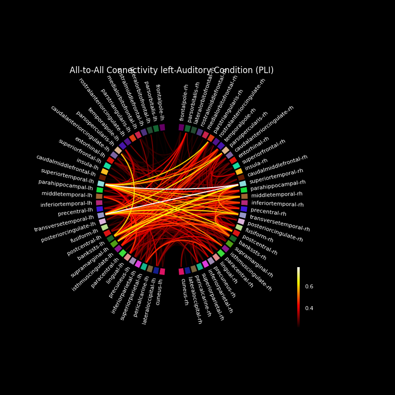
Now, we visualize this connectivity using a circular graph layout.
# First, we reorder the labels based on their location in the left hemi
label_names = [label.name for label in labels]

lh_labels = [name for name in label_names if name.endswith('lh')]

# Get the y-location of the label
label_ypos = list()
for name in lh_labels:
    idx = label_names.index(name)
    ypos = np.mean(labels[idx].pos[:, 1])
    label_ypos.append(ypos)

# Reorder the labels based on their location
lh_labels = [label for (yp, label) in sorted(zip(label_ypos, lh_labels))]

# For the right hemi
rh_labels = [label[:-2] + 'rh' for label in lh_labels]

# Save the plot order and create a circular layout
node_order = list()
node_order.extend(lh_labels[::-1])  # reverse the order
node_order.extend(rh_labels)

node_angles = circular_layout(label_names, node_order, start_pos=90,
                              group_boundaries=[0, len(label_names) / 2])

# Plot the graph using node colors from the FreeSurfer parcellation. We only
# show the 300 strongest connections.
plot_connectivity_circle(con_res['pli'], label_names, n_lines=300,
                         node_angles=node_angles, node_colors=label_colors,
                         title='All-to-All Connectivity left-Auditory '
                               'Condition (PLI)')
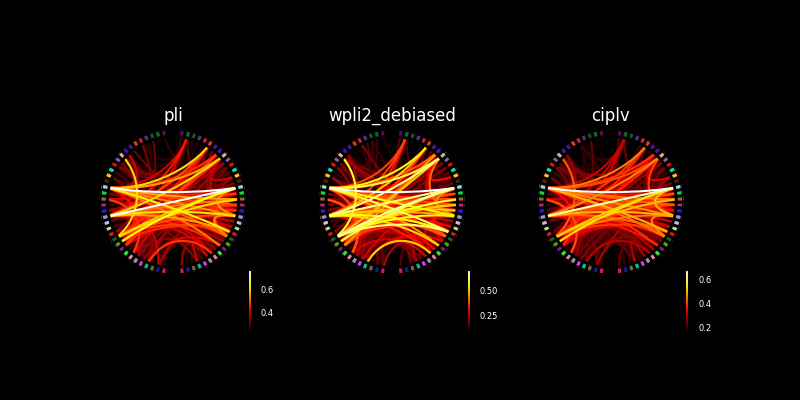
Make two connectivity plots in the same figure
We can also assign these connectivity plots to axes in a figure. Below we’ll show the connectivity plot using two different connectivity methods.
fig = plt.figure(num=None, figsize=(8, 4), facecolor='black')
no_names = [''] * len(label_names)
for ii, method in enumerate(con_methods):
    plot_connectivity_circle(con_res[method], no_names, n_lines=300,
                             node_angles=node_angles, node_colors=label_colors,
                             title=method, padding=0, fontsize_colorbar=6,
                             fig=fig, subplot=(1, 3, ii + 1))

plt.show()
Save the figure (optional)
By default matplotlib does not save using the facecolor, even though this was set when the figure was generated. If not set via savefig, the labels, title, and legend will be cut off from the output png file.
# fname_fig = data_path + '/MEG/sample/plot_inverse_connect.png'
# fig.savefig(fname_fig, facecolor='black')
Total running time of the script: ( 0 minutes 8.478 seconds)
Estimated memory usage: 8 MB