Note
Click here to download the full example code
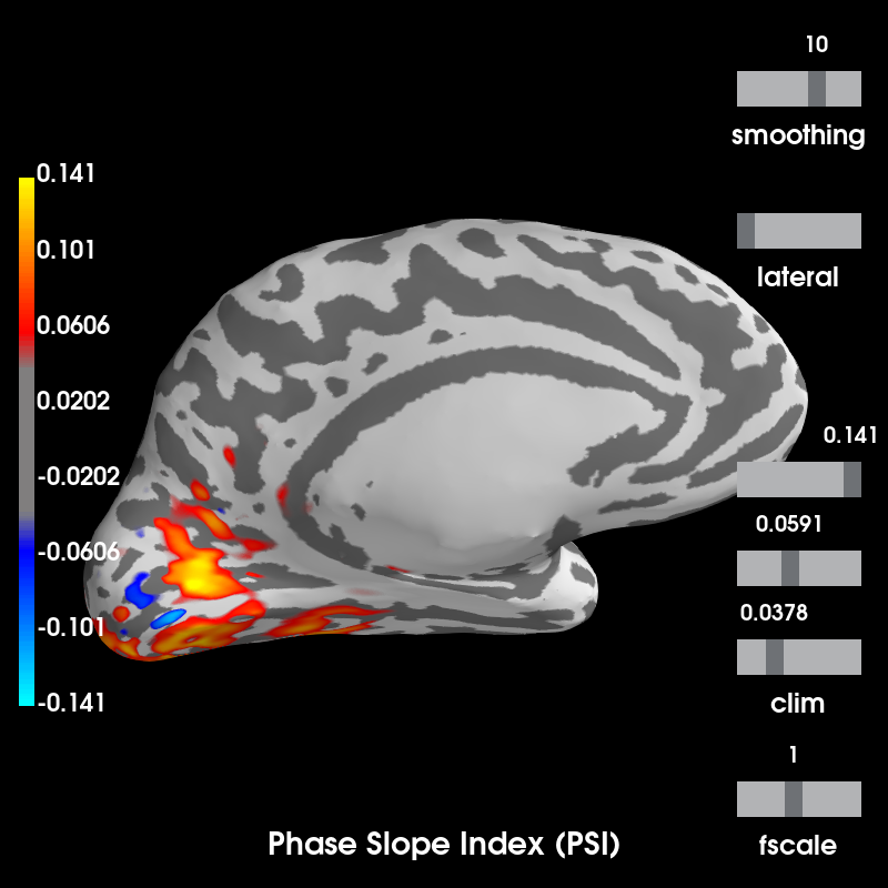
Compute Phase Slope Index (PSI) in source space for a visual stimulus
This example demonstrates how the phase slope index (PSI) 1 can be computed in source space based on single trial dSPM source estimates. In addition, the example shows advanced usage of the connectivity estimation routines by first extracting a label time course for each epoch and then combining the label time course with the single trial source estimates to compute the connectivity.
The result clearly shows how the activity in the visual label precedes more widespread activity (as a postivive PSI means the label time course is leading).
References
- 1
Nolte et al. “Robustly Estimating the Flow Direction of Information in Complex Physical Systems”, Physical Review Letters, vol. 100, no. 23, pp. 1-4, Jun. 2008.
Out:
Reading inverse operator decomposition from /home/circleci/mne_data/MNE-sample-data/MEG/sample/sample_audvis-meg-oct-6-meg-inv.fif...
    Reading inverse operator info...
    [done]
    Reading inverse operator decomposition...
    [done]
    305 x 305 full covariance (kind = 1) found.
    Read a total of 4 projection items:
        PCA-v1 (1 x 10²) active
        PCA-v2 (1 x 10²) active
        PCA-v3 (1 x 10²) active
        Average EEG reference (1 x 60) active
    Noise covariance matrix read.
    22494 x 22494 diagonal covariance (kind = 2) found.
    Source covariance matrix read.
    22494 x 22494 diagonal covariance (kind = 6) found.
    Orientation priors read.
    22494 x 22494 diagonal covariance (kind = 5) found.
    Depth priors read.
    Did not find the desired covariance matrix (kind = 3)
    Reading a source space...
    Computing patch statistics...
    Patch information added...
    Distance information added...
    [done]
    Reading a source space...
    Computing patch statistics...
    Patch information added...
    Distance information added...
    [done]
    2 source spaces read
    Read a total of 4 projection items:
        PCA-v1 (1 x 10²) active
        PCA-v2 (1 x 10²) active
        PCA-v3 (1 x 10²) active
        Average EEG reference (1 x 60) active
    Source spaces transformed to the inverse solution coordinate frame
Opening raw data file /home/circleci/mne_data/MNE-sample-data/MEG/sample/sample_audvis_filt-0-40_raw.fif...
    Read a total of 4 projection items:
        PCA-v1 (1 x 10²)  idle
        PCA-v2 (1 x 10²)  idle
        PCA-v3 (1 x 10²)  idle
        Average EEG reference (1 x 60)  idle
    Range : 6450 ... 48149 =     42.956 ...   320.665 secs
Ready.
Reading 0 ... 41699  =      0.000 ...   277.709 secs...
Not setting metadata
Not setting metadata
70 matching events found
Applying baseline correction (mode: mean)
Created an SSP operator (subspace dimension = 3)
4 projection items activated
Preparing the inverse operator for use...
    Scaled noise and source covariance from nave = 1 to nave = 1
    Created the regularized inverter
    Created an SSP operator (subspace dimension = 3)
    Created the whitener using a noise covariance matrix with rank 302 (3 small eigenvalues omitted)
    Computing noise-normalization factors (dSPM)...
[done]
Picked 305 channels from the data
Computing inverse...
    Eigenleads need to be weighted ...
Processing epoch : 1 / 70 (at most)
Processing epoch : 2 / 70 (at most)
Processing epoch : 3 / 70 (at most)
Processing epoch : 4 / 70 (at most)
Processing epoch : 5 / 70 (at most)
Processing epoch : 6 / 70 (at most)
Processing epoch : 7 / 70 (at most)
    Rejecting  epoch based on EOG : ['EOG 061']
Processing epoch : 8 / 70 (at most)
Processing epoch : 9 / 70 (at most)
Processing epoch : 10 / 70 (at most)
Processing epoch : 11 / 70 (at most)
    Rejecting  epoch based on EOG : ['EOG 061']
Processing epoch : 12 / 70 (at most)
Processing epoch : 13 / 70 (at most)
Processing epoch : 14 / 70 (at most)
Processing epoch : 15 / 70 (at most)
    Rejecting  epoch based on EOG : ['EOG 061']
Processing epoch : 16 / 70 (at most)
Processing epoch : 17 / 70 (at most)
Processing epoch : 18 / 70 (at most)
Processing epoch : 19 / 70 (at most)
    Rejecting  epoch based on EOG : ['EOG 061']
Processing epoch : 20 / 70 (at most)
Processing epoch : 21 / 70 (at most)
Processing epoch : 22 / 70 (at most)
Processing epoch : 23 / 70 (at most)
Processing epoch : 24 / 70 (at most)
Processing epoch : 25 / 70 (at most)
    Rejecting  epoch based on EOG : ['EOG 061']
Processing epoch : 26 / 70 (at most)
Processing epoch : 27 / 70 (at most)
    Rejecting  epoch based on EOG : ['EOG 061']
Processing epoch : 28 / 70 (at most)
Processing epoch : 29 / 70 (at most)
Processing epoch : 30 / 70 (at most)
Processing epoch : 31 / 70 (at most)
Processing epoch : 32 / 70 (at most)
Processing epoch : 33 / 70 (at most)
Processing epoch : 34 / 70 (at most)
    Rejecting  epoch based on EOG : ['EOG 061']
Processing epoch : 35 / 70 (at most)
Processing epoch : 36 / 70 (at most)
Processing epoch : 37 / 70 (at most)
Processing epoch : 38 / 70 (at most)
    Rejecting  epoch based on EOG : ['EOG 061']
Processing epoch : 39 / 70 (at most)
    Rejecting  epoch based on EOG : ['EOG 061']
Processing epoch : 40 / 70 (at most)
Processing epoch : 41 / 70 (at most)
Processing epoch : 42 / 70 (at most)
Processing epoch : 43 / 70 (at most)
Processing epoch : 44 / 70 (at most)
Processing epoch : 45 / 70 (at most)
    Rejecting  epoch based on EOG : ['EOG 061']
Processing epoch : 46 / 70 (at most)
Processing epoch : 47 / 70 (at most)
Processing epoch : 48 / 70 (at most)
Processing epoch : 49 / 70 (at most)
Processing epoch : 50 / 70 (at most)
    Rejecting  epoch based on EOG : ['EOG 061']
    Rejecting  epoch based on EOG : ['EOG 061']
    Rejecting  epoch based on EOG : ['EOG 061']
Processing epoch : 51 / 70 (at most)
Processing epoch : 52 / 70 (at most)
Processing epoch : 53 / 70 (at most)
Processing epoch : 54 / 70 (at most)
Processing epoch : 55 / 70 (at most)
    Rejecting  epoch based on EOG : ['EOG 061']
Processing epoch : 56 / 70 (at most)
Estimating phase slope index (PSI)
Connectivity computation...
    computing connectivity for 7498 connections
    using t=0.000s..0.499s for estimation (76 points)
    frequencies: 11.9Hz..19.8Hz (5 points)
    Using multitaper spectrum estimation with 7 DPSS windows
    the following metrics will be computed: Coherency
    computing connectivity for epoch 1
    computing connectivity for epoch 2
    computing connectivity for epoch 3
    computing connectivity for epoch 4
    computing connectivity for epoch 5
    computing connectivity for epoch 6
    computing connectivity for epoch 7
    computing connectivity for epoch 8
    computing connectivity for epoch 9
    computing connectivity for epoch 10
    computing connectivity for epoch 11
    computing connectivity for epoch 12
    computing connectivity for epoch 13
    computing connectivity for epoch 14
    computing connectivity for epoch 15
    computing connectivity for epoch 16
    computing connectivity for epoch 17
    computing connectivity for epoch 18
    computing connectivity for epoch 19
    computing connectivity for epoch 20
    computing connectivity for epoch 21
    computing connectivity for epoch 22
    computing connectivity for epoch 23
    computing connectivity for epoch 24
    computing connectivity for epoch 25
    computing connectivity for epoch 26
    computing connectivity for epoch 27
    computing connectivity for epoch 28
    computing connectivity for epoch 29
    computing connectivity for epoch 30
    computing connectivity for epoch 31
    computing connectivity for epoch 32
    computing connectivity for epoch 33
    computing connectivity for epoch 34
    computing connectivity for epoch 35
    computing connectivity for epoch 36
    computing connectivity for epoch 37
    computing connectivity for epoch 38
    computing connectivity for epoch 39
    computing connectivity for epoch 40
    computing connectivity for epoch 41
    computing connectivity for epoch 42
    computing connectivity for epoch 43
    computing connectivity for epoch 44
    computing connectivity for epoch 45
    computing connectivity for epoch 46
    computing connectivity for epoch 47
    computing connectivity for epoch 48
    computing connectivity for epoch 49
    computing connectivity for epoch 50
    computing connectivity for epoch 51
    computing connectivity for epoch 52
    computing connectivity for epoch 53
    computing connectivity for epoch 54
    computing connectivity for epoch 55
    computing connectivity for epoch 56
[Connectivity computation done]
Computing PSI from estimated Coherency
[PSI Estimation Done]
Using control points [0.03784692 0.0590657  0.1413717 ]
# Author: Martin Luessi <mluessi@nmr.mgh.harvard.edu>
#
# License: BSD (3-clause)


import numpy as np

import mne
from mne.datasets import sample
from mne.minimum_norm import read_inverse_operator, apply_inverse_epochs
from mne.connectivity import seed_target_indices, phase_slope_index

print(__doc__)

data_path = sample.data_path()
subjects_dir = data_path + '/subjects'
fname_inv = data_path + '/MEG/sample/sample_audvis-meg-oct-6-meg-inv.fif'
fname_raw = data_path + '/MEG/sample/sample_audvis_filt-0-40_raw.fif'
fname_event = data_path + '/MEG/sample/sample_audvis_filt-0-40_raw-eve.fif'
fname_label = data_path + '/MEG/sample/labels/Vis-lh.label'

event_id, tmin, tmax = 4, -0.2, 0.5
method = "dSPM"  # use dSPM method (could also be MNE or sLORETA)

# Load data
inverse_operator = read_inverse_operator(fname_inv)
raw = mne.io.read_raw_fif(fname_raw, preload=True)
events = mne.read_events(fname_event)

# pick MEG channels
picks = mne.pick_types(raw.info, meg=True, eeg=False, stim=False, eog=True,
                       exclude='bads')

# Read epochs
epochs = mne.Epochs(raw, events, event_id, tmin, tmax, picks=picks,
                    baseline=(None, 0), reject=dict(mag=4e-12, grad=4000e-13,
                                                    eog=150e-6))

# Compute inverse solution and for each epoch. Note that since we are passing
# the output to both extract_label_time_course and the phase_slope_index
# functions, we have to use "return_generator=False", since it is only possible
# to iterate over generators once.
snr = 1.0  # use lower SNR for single epochs
lambda2 = 1.0 / snr ** 2
stcs = apply_inverse_epochs(epochs, inverse_operator, lambda2, method,
                            pick_ori="normal", return_generator=True)

# Now, we generate seed time series by averaging the activity in the left
# visual corex
label = mne.read_label(fname_label)
src = inverse_operator['src']  # the source space used
seed_ts = mne.extract_label_time_course(stcs, label, src, mode='mean_flip',
                                        verbose='error')

# Combine the seed time course with the source estimates. There will be a total
# of 7500 signals:
# index 0: time course extracted from label
# index 1..7499: dSPM source space time courses
stcs = apply_inverse_epochs(epochs, inverse_operator, lambda2, method,
                            pick_ori="normal", return_generator=True)
comb_ts = list(zip(seed_ts, stcs))

# Construct indices to estimate connectivity between the label time course
# and all source space time courses
vertices = [src[i]['vertno'] for i in range(2)]
n_signals_tot = 1 + len(vertices[0]) + len(vertices[1])

indices = seed_target_indices([0], np.arange(1, n_signals_tot))

# Compute the PSI in the frequency range 10Hz-20Hz. We exclude the baseline
# period from the connectivity estimation.
fmin = 10.
fmax = 20.
tmin_con = 0.
sfreq = epochs.info['sfreq']  # the sampling frequency

psi, freqs, times, n_epochs, _ = phase_slope_index(
    comb_ts, mode='multitaper', indices=indices, sfreq=sfreq,
    fmin=fmin, fmax=fmax, tmin=tmin_con)

# Generate a SourceEstimate with the PSI. This is simple since we used a single
# seed (inspect the indices variable to see how the PSI scores are arranged in
# the output)
psi_stc = mne.SourceEstimate(psi, vertices=vertices, tmin=0, tstep=1,
                             subject='sample')

# Now we can visualize the PSI using the :meth:`~mne.SourceEstimate.plot`
# method. We use a custom colormap to show signed values
v_max = np.max(np.abs(psi))
brain = psi_stc.plot(surface='inflated', hemi='lh',
                     time_label='Phase Slope Index (PSI)',
                     subjects_dir=subjects_dir,
                     clim=dict(kind='percent', pos_lims=(95, 97.5, 100)))
brain.show_view('medial')
brain.add_label(fname_label, color='green', alpha=0.7)
Total running time of the script: ( 0 minutes 15.964 seconds)
Estimated memory usage: 148 MB