Decoding sensor space data with generalization across time and conditions¶

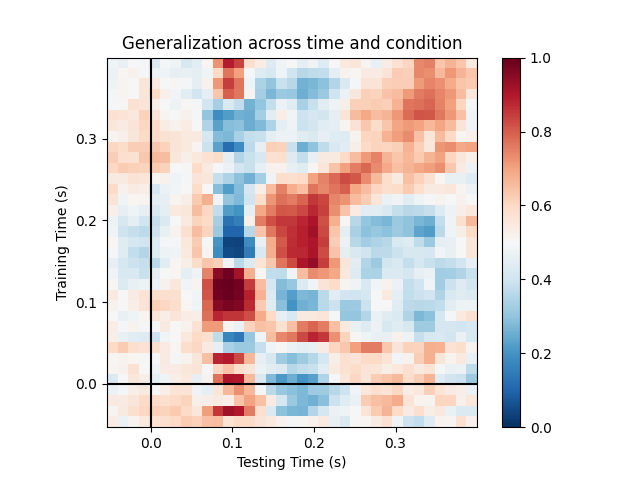
This example runs the analysis described in 1. It illustrates how one can fit a linear classifier to identify a discriminatory topography at a given time instant and subsequently assess whether this linear model can accurately predict all of the time samples of a second set of conditions.

References¶

1: King & Dehaene (2014) ‘Characterizing the dynamics of mental representations: the Temporal Generalization method’, Trends In Cognitive Sciences, 18(4), 203-210. doi: 10.1016/j.tics.2014.01.002.

# Authors: Jean-Remi King <jeanremi.king@gmail.com>
#          Alexandre Gramfort <alexandre.gramfort@inria.fr>
#          Denis Engemann <denis.engemann@gmail.com>
#
# License: BSD (3-clause)

import matplotlib.pyplot as plt

from sklearn.pipeline import make_pipeline
from sklearn.preprocessing import StandardScaler
from sklearn.linear_model import LogisticRegression

import mne
from mne.datasets import sample
from mne.decoding import GeneralizingEstimator

print(__doc__)

# Preprocess data
data_path = sample.data_path()
# Load and filter data, set up epochs
raw_fname = data_path + '/MEG/sample/sample_audvis_filt-0-40_raw.fif'
events_fname = data_path + '/MEG/sample/sample_audvis_filt-0-40_raw-eve.fif'
raw = mne.io.read_raw_fif(raw_fname, preload=True)
picks = mne.pick_types(raw.info, meg=True, exclude='bads')  # Pick MEG channels
raw.filter(1., 30., fir_design='firwin')  # Band pass filtering signals
events = mne.read_events(events_fname)
event_id = {'Auditory/Left': 1, 'Auditory/Right': 2,
            'Visual/Left': 3, 'Visual/Right': 4}
tmin = -0.050
tmax = 0.400
# decimate to make the example faster to run, but then use verbose='error' in
# the Epochs constructor to suppress warning about decimation causing aliasing
decim = 2
epochs = mne.Epochs(raw, events, event_id=event_id, tmin=tmin, tmax=tmax,
                    proj=True, picks=picks, baseline=None, preload=True,
                    reject=dict(mag=5e-12), decim=decim, verbose='error')

Out:

Opening raw data file /home/circleci/mne_data/MNE-sample-data/MEG/sample/sample_audvis_filt-0-40_raw.fif...
    Read a total of 4 projection items:
        PCA-v1 (1 x 102)  idle
        PCA-v2 (1 x 102)  idle
        PCA-v3 (1 x 102)  idle
        Average EEG reference (1 x 60)  idle
    Range : 6450 ... 48149 =     42.956 ...   320.665 secs
Ready.
Reading 0 ... 41699  =      0.000 ...   277.709 secs...
Filtering raw data in 1 contiguous segment
Setting up band-pass filter from 1 - 30 Hz

FIR filter parameters
---------------------
Designing a one-pass, zero-phase, non-causal bandpass filter:
- Windowed time-domain design (firwin) method
- Hamming window with 0.0194 passband ripple and 53 dB stopband attenuation
- Lower passband edge: 1.00
- Lower transition bandwidth: 1.00 Hz (-6 dB cutoff frequency: 0.50 Hz)
- Upper passband edge: 30.00 Hz
- Upper transition bandwidth: 7.50 Hz (-6 dB cutoff frequency: 33.75 Hz)
- Filter length: 497 samples (3.310 sec)

We will train the classifier on all left visual vs auditory trials and test on all right visual vs auditory trials.

clf = make_pipeline(StandardScaler(), LogisticRegression(solver='lbfgs'))
time_gen = GeneralizingEstimator(clf, scoring='roc_auc', n_jobs=1,
                                 verbose=True)

# Fit classifiers on the epochs where the stimulus was presented to the left.
# Note that the experimental condition y indicates auditory or visual
time_gen.fit(X=epochs['Left'].get_data(),
             y=epochs['Left'].events[:, 2] > 2)

Out:

  0%|          | Fitting GeneralizingEstimator : 0/35 [00:00<?,       ?it/s]
  6%|5         | Fitting GeneralizingEstimator : 2/35 [00:00<00:00,   46.67it/s]
 11%|#1        | Fitting GeneralizingEstimator : 4/35 [00:00<00:00,   47.08it/s]
 17%|#7        | Fitting GeneralizingEstimator : 6/35 [00:00<00:00,   47.27it/s]
 23%|##2       | Fitting GeneralizingEstimator : 8/35 [00:00<00:00,   47.69it/s]
 31%|###1      | Fitting GeneralizingEstimator : 11/35 [00:00<00:00,   48.51it/s]
 43%|####2     | Fitting GeneralizingEstimator : 15/35 [00:00<00:00,   49.74it/s]
 51%|#####1    | Fitting GeneralizingEstimator : 18/35 [00:00<00:00,   50.85it/s]
 60%|######    | Fitting GeneralizingEstimator : 21/35 [00:00<00:00,   51.70it/s]
 66%|######5   | Fitting GeneralizingEstimator : 23/35 [00:00<00:00,   51.91it/s]
 74%|#######4  | Fitting GeneralizingEstimator : 26/35 [00:00<00:00,   52.98it/s]
 80%|########  | Fitting GeneralizingEstimator : 28/35 [00:00<00:00,   53.26it/s]
 89%|########8 | Fitting GeneralizingEstimator : 31/35 [00:00<00:00,   53.87it/s]
 94%|#########4| Fitting GeneralizingEstimator : 33/35 [00:00<00:00,   53.80it/s]
100%|##########| Fitting GeneralizingEstimator : 35/35 [00:00<00:00,   55.18it/s]
100%|##########| Fitting GeneralizingEstimator : 35/35 [00:00<00:00,   68.16it/s]

Score on the epochs where the stimulus was presented to the right.

scores = time_gen.score(X=epochs['Right'].get_data(),
                        y=epochs['Right'].events[:, 2] > 2)

Out:

  0%|          | Scoring GeneralizingEstimator : 0/1225 [00:00<?,       ?it/s]
  2%|1         | Scoring GeneralizingEstimator : 21/1225 [00:00<00:01,  613.39it/s]
  4%|3         | Scoring GeneralizingEstimator : 46/1225 [00:00<00:01,  618.32it/s]
  6%|5         | Scoring GeneralizingEstimator : 72/1225 [00:00<00:01,  624.50it/s]
  8%|7         | Scoring GeneralizingEstimator : 97/1225 [00:00<00:01,  629.41it/s]
 10%|#         | Scoring GeneralizingEstimator : 123/1225 [00:00<00:01,  635.19it/s]
 12%|#2        | Scoring GeneralizingEstimator : 149/1225 [00:00<00:01,  640.70it/s]
 14%|#4        | Scoring GeneralizingEstimator : 174/1225 [00:00<00:01,  645.07it/s]
 16%|#6        | Scoring GeneralizingEstimator : 200/1225 [00:00<00:01,  650.17it/s]
 18%|#8        | Scoring GeneralizingEstimator : 225/1225 [00:00<00:01,  654.13it/s]
 20%|##        | Scoring GeneralizingEstimator : 251/1225 [00:00<00:01,  659.11it/s]
 23%|##2       | Scoring GeneralizingEstimator : 276/1225 [00:00<00:01,  662.67it/s]
 25%|##4       | Scoring GeneralizingEstimator : 302/1225 [00:00<00:01,  667.27it/s]
 27%|##6       | Scoring GeneralizingEstimator : 328/1225 [00:00<00:01,  671.43it/s]
 29%|##8       | Scoring GeneralizingEstimator : 353/1225 [00:00<00:01,  674.38it/s]
 31%|###       | Scoring GeneralizingEstimator : 379/1225 [00:00<00:01,  678.44it/s]
 33%|###2      | Scoring GeneralizingEstimator : 404/1225 [00:00<00:01,  681.28it/s]
 35%|###5      | Scoring GeneralizingEstimator : 430/1225 [00:00<00:01,  685.05it/s]
 37%|###7      | Scoring GeneralizingEstimator : 456/1225 [00:00<00:01,  688.81it/s]
 39%|###9      | Scoring GeneralizingEstimator : 482/1225 [00:00<00:01,  692.51it/s]
 41%|####1     | Scoring GeneralizingEstimator : 508/1225 [00:00<00:01,  695.96it/s]
 44%|####3     | Scoring GeneralizingEstimator : 534/1225 [00:00<00:00,  699.29it/s]
 46%|####5     | Scoring GeneralizingEstimator : 560/1225 [00:00<00:00,  702.33it/s]
 48%|####7     | Scoring GeneralizingEstimator : 586/1225 [00:00<00:00,  705.29it/s]
 50%|####9     | Scoring GeneralizingEstimator : 612/1225 [00:00<00:00,  708.18it/s]
 52%|#####2    | Scoring GeneralizingEstimator : 638/1225 [00:00<00:00,  711.00it/s]
 54%|#####4    | Scoring GeneralizingEstimator : 663/1225 [00:00<00:00,  712.30it/s]
 56%|#####6    | Scoring GeneralizingEstimator : 689/1225 [00:00<00:00,  714.91it/s]
 58%|#####8    | Scoring GeneralizingEstimator : 715/1225 [00:00<00:00,  717.30it/s]
 60%|######    | Scoring GeneralizingEstimator : 741/1225 [00:00<00:00,  719.69it/s]
 63%|######2   | Scoring GeneralizingEstimator : 767/1225 [00:01<00:00,  722.03it/s]
 65%|######4   | Scoring GeneralizingEstimator : 793/1225 [00:01<00:00,  724.25it/s]
 67%|######6   | Scoring GeneralizingEstimator : 819/1225 [00:01<00:00,  726.38it/s]
 69%|######8   | Scoring GeneralizingEstimator : 845/1225 [00:01<00:00,  728.41it/s]
 71%|#######1  | Scoring GeneralizingEstimator : 871/1225 [00:01<00:00,  730.32it/s]
 73%|#######3  | Scoring GeneralizingEstimator : 897/1225 [00:01<00:00,  732.14it/s]
 75%|#######5  | Scoring GeneralizingEstimator : 923/1225 [00:01<00:00,  733.71it/s]
 77%|#######7  | Scoring GeneralizingEstimator : 949/1225 [00:01<00:00,  735.33it/s]
 80%|#######9  | Scoring GeneralizingEstimator : 975/1225 [00:01<00:00,  736.96it/s]
 82%|########1 | Scoring GeneralizingEstimator : 1001/1225 [00:01<00:00,  738.49it/s]
 84%|########3 | Scoring GeneralizingEstimator : 1027/1225 [00:01<00:00,  739.93it/s]
 86%|########5 | Scoring GeneralizingEstimator : 1053/1225 [00:01<00:00,  741.22it/s]
 88%|########8 | Scoring GeneralizingEstimator : 1079/1225 [00:01<00:00,  742.44it/s]
 90%|######### | Scoring GeneralizingEstimator : 1105/1225 [00:01<00:00,  743.70it/s]
 92%|#########2| Scoring GeneralizingEstimator : 1131/1225 [00:01<00:00,  744.84it/s]
 94%|#########4| Scoring GeneralizingEstimator : 1157/1225 [00:01<00:00,  745.90it/s]
 97%|#########6| Scoring GeneralizingEstimator : 1183/1225 [00:01<00:00,  747.03it/s]
 99%|#########8| Scoring GeneralizingEstimator : 1209/1225 [00:01<00:00,  748.03it/s]
100%|##########| Scoring GeneralizingEstimator : 1225/1225 [00:01<00:00,  749.18it/s]
100%|##########| Scoring GeneralizingEstimator : 1225/1225 [00:01<00:00,  759.42it/s]

Plot

fig, ax = plt.subplots(1)
im = ax.matshow(scores, vmin=0, vmax=1., cmap='RdBu_r', origin='lower',
                extent=epochs.times[[0, -1, 0, -1]])
ax.axhline(0., color='k')
ax.axvline(0., color='k')
ax.xaxis.set_ticks_position('bottom')
ax.set_xlabel('Testing Time (s)')
ax.set_ylabel('Training Time (s)')
ax.set_title('Generalization across time and condition')
plt.colorbar(im, ax=ax)
plt.show()