Note
Click here to download the full example code
Compute sLORETA inverse solution on raw data
Compute sLORETA inverse solution on raw dataset restricted to a brain label and stores the solution in stc files for visualisation.
# Author: Alexandre Gramfort <alexandre.gramfort@inria.fr>
#
# License: BSD (3-clause)

import matplotlib.pyplot as plt

import mne
from mne.datasets import sample
from mne.minimum_norm import apply_inverse_raw, read_inverse_operator

print(__doc__)

data_path = sample.data_path()
fname_inv = data_path + '/MEG/sample/sample_audvis-meg-oct-6-meg-inv.fif'
fname_raw = data_path + '/MEG/sample/sample_audvis_raw.fif'
label_name = 'Aud-lh'
fname_label = data_path + '/MEG/sample/labels/%s.label' % label_name

snr = 1.0  # use smaller SNR for raw data
lambda2 = 1.0 / snr ** 2
method = "sLORETA"  # use sLORETA method (could also be MNE or dSPM)

# Load data
raw = mne.io.read_raw_fif(fname_raw)
inverse_operator = read_inverse_operator(fname_inv)
label = mne.read_label(fname_label)

raw.set_eeg_reference('average', projection=True)  # set average reference.
start, stop = raw.time_as_index([0, 15])  # read the first 15s of data

# Compute inverse solution
stc = apply_inverse_raw(raw, inverse_operator, lambda2, method, label,
                        start, stop, pick_ori=None)

# Save result in stc files
stc.save('mne_%s_raw_inverse_%s' % (method, label_name))
Out:
Opening raw data file /home/circleci/mne_data/MNE-sample-data/MEG/sample/sample_audvis_raw.fif...
    Read a total of 3 projection items:
        PCA-v1 (1 x 10²)  idle
        PCA-v2 (1 x 10²)  idle
        PCA-v3 (1 x 10²)  idle
    Range : 25800 ... 192599 =     42.956 ...   320.670 secs
Ready.
Reading inverse operator decomposition from /home/circleci/mne_data/MNE-sample-data/MEG/sample/sample_audvis-meg-oct-6-meg-inv.fif...
    Reading inverse operator info...
    [done]
    Reading inverse operator decomposition...
    [done]
    305 x 305 full covariance (kind = 1) found.
    Read a total of 4 projection items:
        PCA-v1 (1 x 10²) active
        PCA-v2 (1 x 10²) active
        PCA-v3 (1 x 10²) active
        Average EEG reference (1 x 60) active
    Noise covariance matrix read.
    22494 x 22494 diagonal covariance (kind = 2) found.
    Source covariance matrix read.
    22494 x 22494 diagonal covariance (kind = 6) found.
    Orientation priors read.
    22494 x 22494 diagonal covariance (kind = 5) found.
    Depth priors read.
    Did not find the desired covariance matrix (kind = 3)
    Reading a source space...
    Computing patch statistics...
    Patch information added...
    Distance information added...
    [done]
    Reading a source space...
    Computing patch statistics...
    Patch information added...
    Distance information added...
    [done]
    2 source spaces read
    Read a total of 4 projection items:
        PCA-v1 (1 x 10²) active
        PCA-v2 (1 x 10²) active
        PCA-v3 (1 x 10²) active
        Average EEG reference (1 x 60) active
    Source spaces transformed to the inverse solution coordinate frame
Adding average EEG reference projection.
1 projection items deactivated
Preparing the inverse operator for use...
    Scaled noise and source covariance from nave = 1 to nave = 1
    Created the regularized inverter
    Created an SSP operator (subspace dimension = 3)
    Created the whitener using a noise covariance matrix with rank 302 (3 small eigenvalues omitted)
    Computing noise-normalization factors (sLORETA)...
[done]
Applying inverse to raw...
    Picked 305 channels from the data
    Computing inverse...
    Eigenleads need to be weighted ...
    combining the current components...
[done]
Writing STC to disk...
[done]
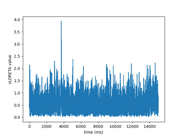
View activation time-series
plt.plot(1e3 * stc.times, stc.data[::100, :].T)
plt.xlabel('time (ms)')
plt.ylabel('%s value' % method)
plt.show()
Total running time of the script: ( 0 minutes 2.213 seconds)
Estimated memory usage: 8 MB