Note
Click here to download the full example code
Annotate muscle artifacts
Muscle contractions produce high frequency activity that can mask brain signal of interest. Muscle artifacts can be produced when clenching the jaw, swallowing, or twitching a cranial muscle. Muscle artifacts are most noticeable in the range of 110-140 Hz.
This example uses annotate_muscle_zscore() to annotate
segments where muscle activity is likely present. This is done by band-pass
filtering the data in the 110-140 Hz range. Then, the envelope is taken using
the hilbert analytical signal to only consider the absolute amplitude and not
the phase of the high frequency signal. The envelope is z-scored and summed
across channels and divided by the square root of the number of channels.
Because muscle artifacts last several hundred milliseconds, a low-pass filter
is applied on the averaged z-scores at 4 Hz, to remove transient peaks.
Segments above a set threshold are annotated as BAD_muscle. In addition,
the min_length_good parameter determines the cutoff for whether short
spans of “good data” in between muscle artifacts are included in the
surrounding “BAD” annotation.
# Authors: Adonay Nunes <adonay.s.nunes@gmail.com>
#          Luke Bloy <luke.bloy@gmail.com>
# License: BSD (3-clause)

import os.path as op
import matplotlib.pyplot as plt
import numpy as np
from mne.datasets.brainstorm import bst_auditory
from mne.io import read_raw_ctf
from mne.preprocessing import annotate_muscle_zscore


# Load data
data_path = bst_auditory.data_path()
raw_fname = op.join(data_path, 'MEG', 'bst_auditory', 'S01_AEF_20131218_01.ds')

raw = read_raw_ctf(raw_fname, preload=False)

raw.crop(130, 160).load_data()  # just use a fraction of data for speed here
raw.resample(300, npad="auto")
Out:
ds directory : /home/circleci/mne_data/MNE-brainstorm-data/bst_auditory/MEG/bst_auditory/S01_AEF_20131218_01.ds
    res4 data read.
    hc data read.
    Separate EEG position data file read.
    Quaternion matching (desired vs. transformed):
       2.51   74.26    0.00 mm <->    2.51   74.26    0.00 mm (orig :  -56.69   50.20 -264.38 mm) diff =    0.000 mm
      -2.51  -74.26    0.00 mm <->   -2.51  -74.26    0.00 mm (orig :   50.89  -52.31 -265.88 mm) diff =    0.000 mm
     108.63    0.00    0.00 mm <->  108.63    0.00   -0.00 mm (orig :   67.41   77.68 -239.53 mm) diff =    0.000 mm
    Coordinate transformations established.
    Reading digitizer points from ['/home/circleci/mne_data/MNE-brainstorm-data/bst_auditory/MEG/bst_auditory/S01_AEF_20131218_01.ds/S01_20131218_01.pos']...
    Polhemus data for 3 HPI coils added
    Device coordinate locations for 3 HPI coils added
    5 extra points added to Polhemus data.
    Measurement info composed.
Finding samples for /home/circleci/mne_data/MNE-brainstorm-data/bst_auditory/MEG/bst_auditory/S01_AEF_20131218_01.ds/S01_AEF_20131218_01.meg4:
    System clock channel is available, checking which samples are valid.
    360 x 2400 = 864000 samples from 340 chs
Current compensation grade : 3
Reading 0 ... 72000  =      0.000 ...    30.000 secs...
4 events found
Event IDs: [64]
23 events found
Event IDs: [1 2]
4 events found
Event IDs: [64]
23 events found
Event IDs: [1 2]
Notch filter the data:
Note
If line noise is present, you should perform notch-filtering before detecting muscle artifacts. See Power line noise for an example.
raw.notch_filter([50, 100])
Out:
Setting up band-stop filter

FIR filter parameters
---------------------
Designing a one-pass, zero-phase, non-causal bandstop filter:
- Windowed time-domain design (firwin) method
- Hamming window with 0.0194 passband ripple and 53 dB stopband attenuation
- Lower transition bandwidth: 0.50 Hz
- Upper transition bandwidth: 0.50 Hz
- Filter length: 1981 samples (6.603 sec)
# The threshold is data dependent, check the optimal threshold by plotting
# ``scores_muscle``.
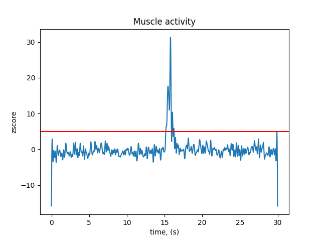
threshold_muscle = 5 # z-score
# Choose one channel type, if there are axial gradiometers and magnetometers,
# select magnetometers as they are more sensitive to muscle activity.
annot_muscle, scores_muscle = annotate_muscle_zscore(
raw, ch_type="mag", threshold=threshold_muscle, min_length_good=0.2,
filter_freq=[110, 140])
Out:
Removing 5 compensators from info because not all compensation channels were picked.
Filtering raw data in 1 contiguous segment
Setting up band-pass filter from 1.1e+02 - 1.4e+02 Hz

FIR filter parameters
---------------------
Designing a one-pass, zero-phase, non-causal bandpass filter:
- Windowed time-domain design (firwin) method
- Hamming window with 0.0194 passband ripple and 53 dB stopband attenuation
- Lower passband edge: 110.00
- Lower transition bandwidth: 27.50 Hz (-6 dB cutoff frequency: 96.25 Hz)
- Upper passband edge: 140.00 Hz
- Upper transition bandwidth: 10.00 Hz (-6 dB cutoff frequency: 145.00 Hz)
- Filter length: 99 samples (0.330 sec)

Setting up low-pass filter at 4 Hz

FIR filter parameters
---------------------
Designing a one-pass, zero-phase, non-causal lowpass filter:
- Windowed time-domain design (firwin) method
- Hamming window with 0.0194 passband ripple and 53 dB stopband attenuation
- Upper passband edge: 4.00 Hz
- Upper transition bandwidth: 2.00 Hz (-6 dB cutoff frequency: 5.00 Hz)
- Filter length: 495 samples (1.650 sec)
Plot muscle z-scores across recording
fig, ax = plt.subplots()
ax.plot(raw.times, scores_muscle)
ax.axhline(y=threshold_muscle, color='r')
ax.set(xlabel='time, (s)', ylabel='zscore', title='Muscle activity')
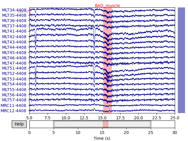
View the annotations
order = np.arange(144, 164)
raw.set_annotations(annot_muscle)
raw.plot(start=5, duration=20, order=order)
Total running time of the script: ( 0 minutes 4.902 seconds)
Estimated memory usage: 195 MB