Note
Click here to download the full example code
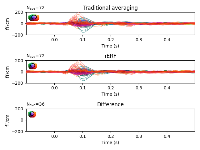
Regression on continuous data (rER[P/F])
This demonstrates how rER[P/F]s - regressing the continuous data - is a generalisation of traditional averaging. If all preprocessing steps are the same, no overlap between epochs exists, and if all predictors are binary, regression is virtually identical to traditional averaging. If overlap exists and/or predictors are continuous, traditional averaging is inapplicable, but regression can estimate effects, including those of continuous predictors.
rERPs are described in: Smith, N. J., & Kutas, M. (2015). Regression-based estimation of ERP waveforms: II. Non-linear effects, overlap correction, and practical considerations. Psychophysiology, 52(2), 169-189.
Out:
Opening raw data file /home/circleci/mne_data/MNE-sample-data/MEG/sample/sample_audvis_filt-0-40_raw.fif...
    Read a total of 4 projection items:
        PCA-v1 (1 x 10²)  idle
        PCA-v2 (1 x 10²)  idle
        PCA-v3 (1 x 10²)  idle
        Average EEG reference (1 x 60)  idle
    Range : 6450 ... 48149 =     42.956 ...   320.665 secs
Ready.
Removing projector <Projection | PCA-v1, active : False, n_channels : 102>
Removing projector <Projection | PCA-v2, active : False, n_channels : 102>
Removing projector <Projection | PCA-v3, active : False, n_channels : 102>
Removing projector <Projection | Average EEG reference, active : False, n_channels : 60>
Reading 0 ... 41699  =      0.000 ...   277.709 secs...
Filtering raw data in 1 contiguous segment
Setting up high-pass filter at 1 Hz

FIR filter parameters
---------------------
Designing a one-pass, zero-phase, non-causal highpass filter:
- Windowed time-domain design (firwin) method
- Hamming window with 0.0194 passband ripple and 53 dB stopband attenuation
- Lower passband edge: 1.00
- Lower transition bandwidth: 1.00 Hz (-6 dB cutoff frequency: 0.50 Hz)
- Filter length: 497 samples (3.310 sec)

319 events found
Event IDs: [ 1  2  3  4  5 32]
# Authors: Jona Sassenhagen <jona.sassenhagen@gmail.de>
#
# License: BSD (3-clause)

import matplotlib.pyplot as plt

import mne
from mne.datasets import sample
from mne.stats.regression import linear_regression_raw

# Load and preprocess data
data_path = sample.data_path()
raw_fname = data_path + '/MEG/sample/sample_audvis_filt-0-40_raw.fif'
raw = mne.io.read_raw_fif(raw_fname)
raw.pick_types(meg='grad', stim=True, eeg=False).load_data()
raw.filter(1, None, fir_design='firwin')  # high-pass

# Set up events
events = mne.find_events(raw)
event_id = {'Aud/L': 1, 'Aud/R': 2}
tmin, tmax = -.1, .5

# regular epoching
picks = mne.pick_types(raw.info, meg=True)
epochs = mne.Epochs(raw, events, event_id, tmin, tmax, reject=None,
                    baseline=None, preload=True, verbose=False)

# rERF
evokeds = linear_regression_raw(raw, events=events, event_id=event_id,
                                reject=None, tmin=tmin, tmax=tmax)
# linear_regression_raw returns a dict of evokeds
# select conditions similarly to mne.Epochs objects

# plot both results, and their difference
cond = "Aud/L"
fig, (ax1, ax2, ax3) = plt.subplots(3, 1)
params = dict(spatial_colors=True, show=False, ylim=dict(grad=(-200, 200)),
              time_unit='s')
epochs[cond].average().plot(axes=ax1, **params)
evokeds[cond].plot(axes=ax2, **params)
contrast = mne.combine_evoked([evokeds[cond], epochs[cond].average()],
                              weights=[1, -1])
contrast.plot(axes=ax3, **params)
ax1.set_title("Traditional averaging")
ax2.set_title("rERF")
ax3.set_title("Difference")
plt.show()
Total running time of the script: ( 0 minutes 3.378 seconds)
Estimated memory usage: 76 MB