How to plot topomaps the way EEGLAB does

If you have previous EEGLAB experience you may have noticed that topomaps (topoplots) generated using MNE-Python look a little different from those created in EEGLAB. If you prefer the EEGLAB style this example will show you how to calculate head sphere origin and radius to obtain EEGLAB-like channel layout in MNE.

# Authors: Mikołaj Magnuski <mmagnuski@swps.edu.pl>
#
# License: BSD (3-clause)
import numpy as np
from matplotlib import pyplot as plt

import mne


print(__doc__)

Create fake data

First we will create a simple evoked object with a single timepoint using biosemi 10-20 channel layout.

biosemi_montage = mne.channels.make_standard_montage('biosemi64')
n_channels = len(biosemi_montage.ch_names)
fake_info = mne.create_info(ch_names=biosemi_montage.ch_names, sfreq=250.,
                            ch_types='eeg')

rng = np.random.RandomState(0)
data = rng.normal(size=(n_channels, 1)) * 1e-6
fake_evoked = mne.EvokedArray(data, fake_info)
fake_evoked.set_montage(biosemi_montage)

Calculate sphere origin and radius

EEGLAB plots head outline at the level where the head circumference is measured in the 10-20 system (a line going through Fpz, T8/T4, Oz and T7/T3 channels). MNE-Python places the head outline lower on the z dimension, at the level of the anatomical landmarks LPA, RPA, and NAS. Therefore to use the EEGLAB layout we have to move the origin of the reference sphere (a sphere that is used as a reference when projecting channel locations to a 2d plane) a few centimeters up.

Instead of approximating this position by eye, as we did in the sensor locations tutorial, here we will calculate it using the position of Fpz, T8, Oz and T7 channels available in our montage.

# first we obtain the 3d positions of selected channels
check_ch = ['Oz', 'Fpz', 'T7', 'T8']
ch_idx = [fake_evoked.ch_names.index(ch) for ch in check_ch]
pos = np.stack([fake_evoked.info['chs'][idx]['loc'][:3] for idx in ch_idx])

# now we calculate the radius from T7 and T8 x position
# (we could use Oz and Fpz y positions as well)
radius = np.abs(pos[[2, 3], 0]).mean()

# then we obtain the x, y, z sphere center this way:
# x: x position of the Oz channel (should be very close to 0)
# y: y position of the T8 channel (should be very close to 0 too)
# z: average z position of Oz, Fpz, T7 and T8 (their z position should be the
#    the same, so we could also use just one of these channels), it should be
#    positive and somewhere around `0.03` (3 cm)
x = pos[0, 0]
y = pos[-1, 1]
z = pos[:, -1].mean()

# lets print the values we got:
print([f'{v:0.5f}' for v in [x, y, z, radius]])

Out:

['0.00000', '0.00000', '0.03683', '0.09494']

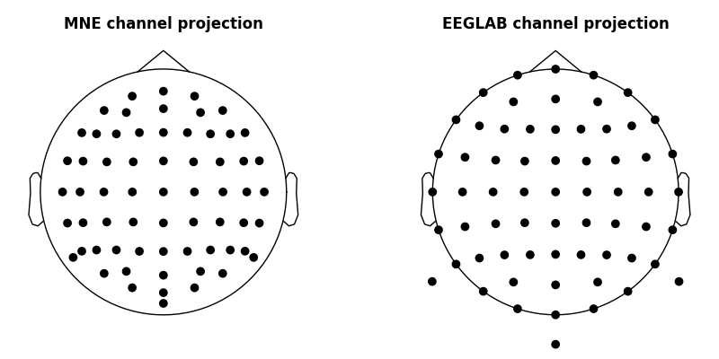
Compare MNE and EEGLAB channel layout

We already have the required x, y, z sphere center and its radius — we can use these values passing them to the sphere argument of many topo-plotting functions (by passing sphere=(x, y, z, radius)).

# create a two-panel figure with some space for the titles at the top
fig, ax = plt.subplots(ncols=2, figsize=(8, 4), gridspec_kw=dict(top=0.9),
                       sharex=True, sharey=True)

# we plot the channel positions with default sphere - the mne way
fake_evoked.plot_sensors(axes=ax[0], show=False)

# in the second panel we plot the positions using the EEGLAB reference sphere
fake_evoked.plot_sensors(sphere=(x, y, z, radius), axes=ax[1], show=False)

# add titles
fig.texts[0].remove()
ax[0].set_title('MNE channel projection', fontweight='bold')
ax[1].set_title('EEGLAB channel projection', fontweight='bold')

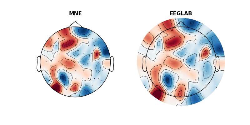
Topomaps (topoplots)

As the last step we do the same, but plotting the topomaps. These will not be particularly interesting as they will show random data but hopefully you will see the difference.

fig, ax = plt.subplots(ncols=2, figsize=(8, 4), gridspec_kw=dict(top=0.9),
                       sharex=True, sharey=True)

mne.viz.plot_topomap(fake_evoked.data[:, 0], fake_evoked.info, axes=ax[0],
                     show=False)
mne.viz.plot_topomap(fake_evoked.data[:, 0], fake_evoked.info, axes=ax[1],
                     show=False, sphere=(x, y, z, radius))

# add titles
ax[0].set_title('MNE', fontweight='bold')
ax[1].set_title('EEGLAB', fontweight='bold')

Estimated memory usage: 8 MB