Working with sensor locations

This tutorial describes how to read and plot sensor locations, and how the physical location of sensors is handled in MNE-Python.

As usual we’ll start by importing the modules we need and loading some example data:

import os
import numpy as np
import matplotlib.pyplot as plt
from mpl_toolkits.mplot3d import Axes3D  # noqa
import mne

sample_data_folder = mne.datasets.sample.data_path()
sample_data_raw_file = os.path.join(sample_data_folder, 'MEG', 'sample',
                                    'sample_audvis_raw.fif')
raw = mne.io.read_raw_fif(sample_data_raw_file, preload=True, verbose=False)

About montages and layouts

Montages contain sensor positions in 3D (x, y, z, in meters), and can be used to set the physical positions of sensors. By specifying the location of sensors relative to the brain, Montages play an important role in computing the forward solution and computing inverse estimates.

In contrast, Layouts are idealized 2-D representations of sensor positions, and are primarily used for arranging individual sensor subplots in a topoplot, or for showing the approximate relative arrangement of sensors as seen from above.

Working with built-in montages

The 3D coordinates of MEG sensors are included in the raw recordings from MEG systems, and are automatically stored in the info attribute of the Raw file upon loading. EEG electrode locations are much more variable because of differences in head shape. Idealized montages for many EEG systems are included during MNE-Python installation; these files are stored in your mne-python directory, in the mne/channels/data/montages folder:

montage_dir = os.path.join(os.path.dirname(mne.__file__),
                           'channels', 'data', 'montages')
print('\nBUILT-IN MONTAGE FILES')
print('======================')
print(sorted(os.listdir(montage_dir)))

Out:

BUILT-IN MONTAGE FILES
======================
['EGI_256.csd', 'GSN-HydroCel-128.sfp', 'GSN-HydroCel-129.sfp', 'GSN-HydroCel-256.sfp', 'GSN-HydroCel-257.sfp', 'GSN-HydroCel-32.sfp', 'GSN-HydroCel-64_1.0.sfp', 'GSN-HydroCel-65_1.0.sfp', 'biosemi128.txt', 'biosemi16.txt', 'biosemi160.txt', 'biosemi256.txt', 'biosemi32.txt', 'biosemi64.txt', 'easycap-M1.txt', 'easycap-M10.txt', 'mgh60.elc', 'mgh70.elc', 'standard_1005.elc', 'standard_1020.elc', 'standard_alphabetic.elc', 'standard_postfixed.elc', 'standard_prefixed.elc', 'standard_primed.elc']

Computing sensor locations

If you are interested in how standard (“idealized”) EEG sensor positions are computed on a spherical head model, the eeg_positions repository provides code and documentation to this end.

These built-in EEG montages can be loaded via mne.channels.make_standard_montage(). Note that when loading via make_standard_montage(), provide the filename without its file extension:

ten_twenty_montage = mne.channels.make_standard_montage('standard_1020')
print(ten_twenty_montage)

Out:

<DigMontage | 0 extras (headshape), 0 HPIs, 3 fiducials, 94 channels>

Once loaded, a montage can be applied to data via one of the instance methods such as raw.set_montage. It is also possible to skip the loading step by passing the filename string directly to the set_montage() method. This won’t work with our sample data, because it’s channel names don’t match the channel names in the standard 10-20 montage, so these commands are not run here:

# these will be equivalent:
# raw_1020 = raw.copy().set_montage(ten_twenty_montage)
# raw_1020 = raw.copy().set_montage('standard_1020')

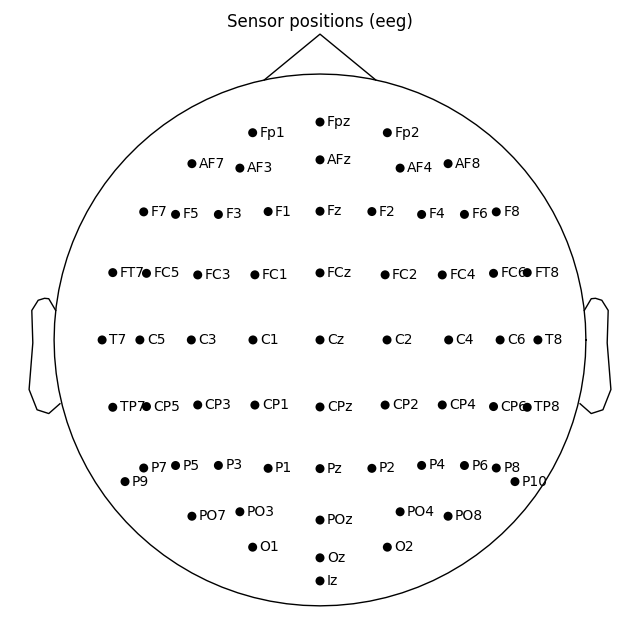
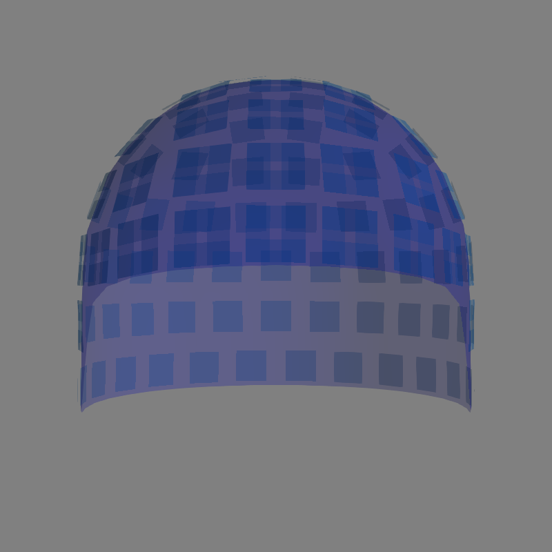
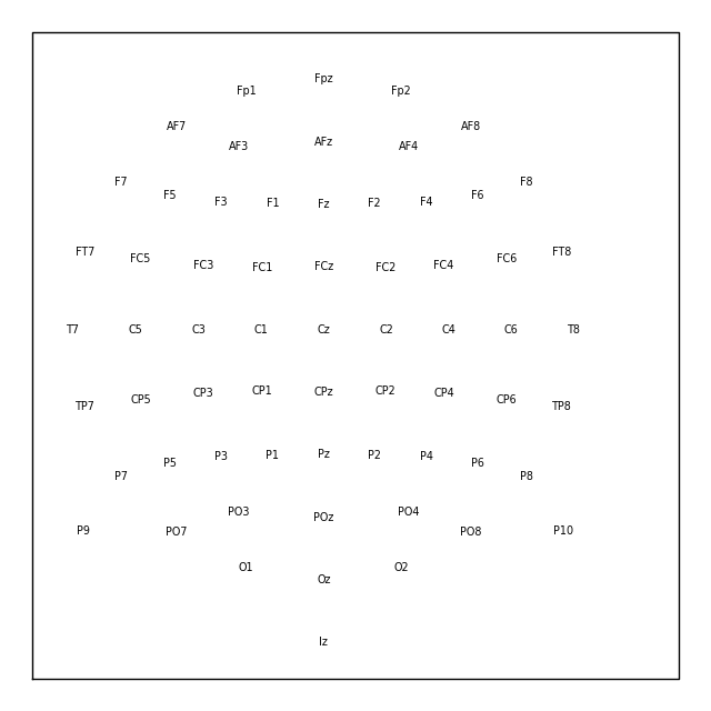
Montage objects have a plot() method for visualization of the sensor locations in 3D; 2D projections are also possible by passing kind='topomap':

fig = ten_twenty_montage.plot(kind='3d')
fig.gca().view_init(azim=70, elev=15)
ten_twenty_montage.plot(kind='topomap', show_names=False)

• 
• 

Out:

4 duplicate electrode labels found:
T7/T3, T8/T4, P7/T5, P8/T6
Plotting 90 unique labels.
Creating RawArray with float64 data, n_channels=90, n_times=1
    Range : 0 ... 0 =      0.000 ...     0.000 secs
Ready.
4 duplicate electrode labels found:
T7/T3, T8/T4, P7/T5, P8/T6
Plotting 90 unique labels.
Creating RawArray with float64 data, n_channels=90, n_times=1
    Range : 0 ... 0 =      0.000 ...     0.000 secs
Ready.

Controlling channel projection (MNE vs EEGLAB)

Channel positions in 2d space are obtained by projecting their actual 3d positions using a sphere as a reference. Because 'standard_1020' montage contains realistic, not spherical, channel positions, we will use a different montage to demonstrate controlling how channels are projected to 2d space.

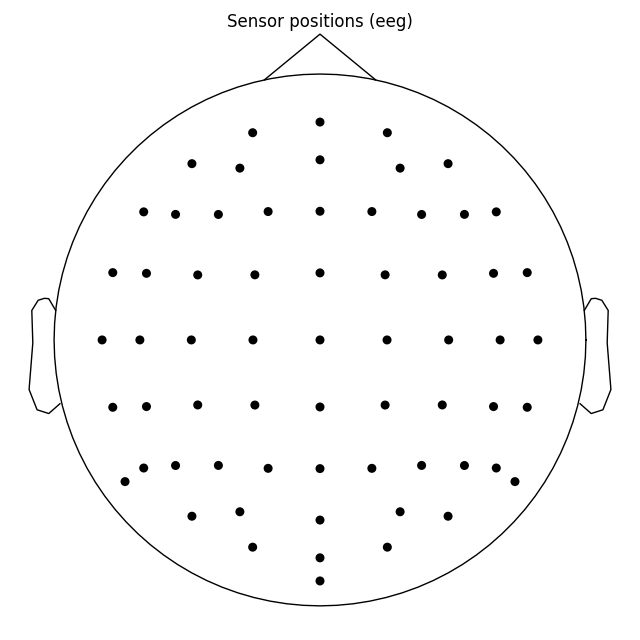
biosemi_montage = mne.channels.make_standard_montage('biosemi64')
biosemi_montage.plot(show_names=False)

Out:

Creating RawArray with float64 data, n_channels=64, n_times=1
    Range : 0 ... 0 =      0.000 ...     0.000 secs
Ready.

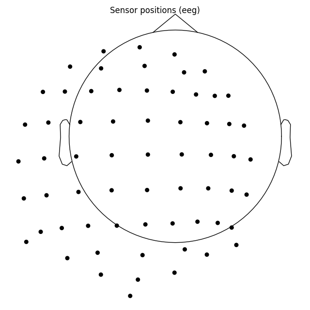
By default a sphere with an origin in (0, 0, 0) x, y, z coordinates and radius of 0.095 meters (9.5 cm) is used. You can use a different sphere radius by passing a single value to sphere argument in any function that plots channels in 2d (like plot() that we use here, but also for example mne.viz.plot_topomap()):

biosemi_montage.plot(show_names=False, sphere=0.07)

Out:

Creating RawArray with float64 data, n_channels=64, n_times=1
    Range : 0 ... 0 =      0.000 ...     0.000 secs
Ready.

To control not only radius, but also the sphere origin, pass a (x, y, z, radius) tuple to sphere argument:

biosemi_montage.plot(show_names=False, sphere=(0.03, 0.02, 0.01, 0.075))

Out:

Creating RawArray with float64 data, n_channels=64, n_times=1
    Range : 0 ... 0 =      0.000 ...     0.000 secs
Ready.

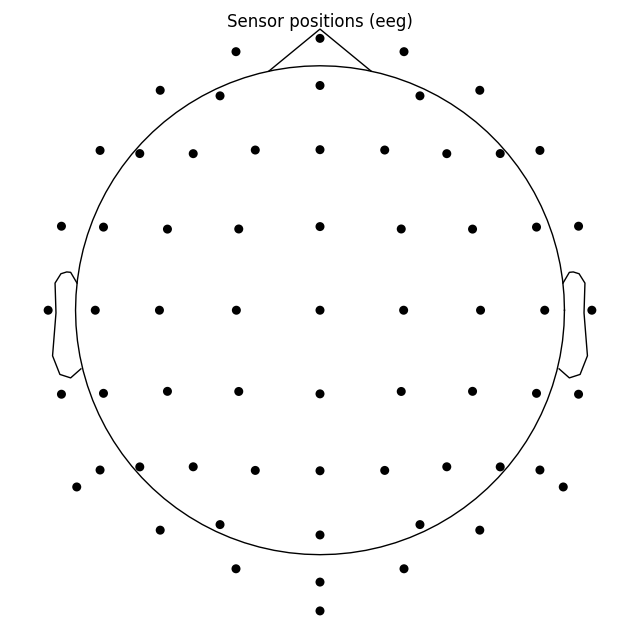
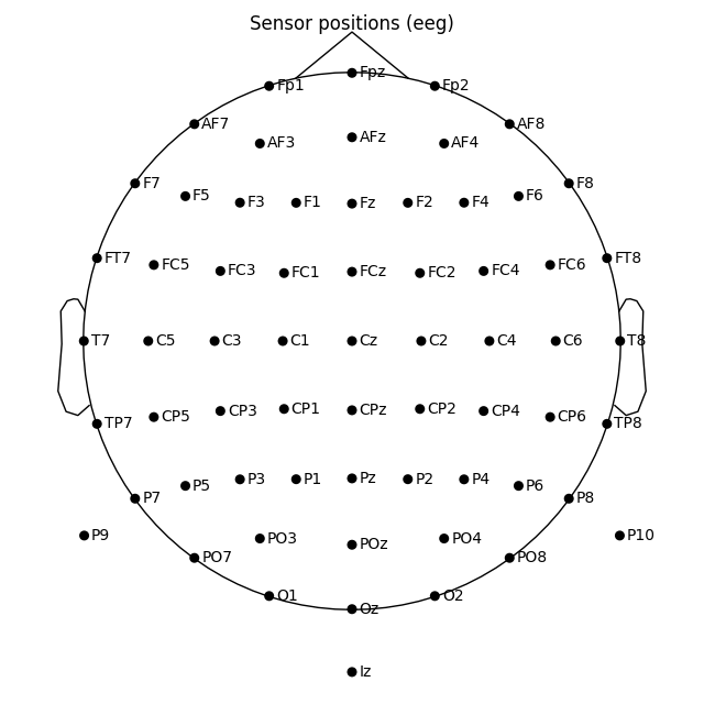
In mne-python the head center and therefore the sphere center are calculated using fiducial points. Because of this the head circle represents head circumference at the nasion and ear level, and not where it is commonly measured in 10-20 EEG system: above nasion at T4/T8, T3/T7, Oz, Fz level. Notice below that by default T7 and Oz channels are placed within the head circle, not on the head outline:

biosemi_montage.plot()

Out:

Creating RawArray with float64 data, n_channels=64, n_times=1
    Range : 0 ... 0 =      0.000 ...     0.000 secs
Ready.

If you have previous EEGLAB experience you may prefer its convention to represent 10-20 head circumference with the head circle. To get EEGLAB-like channel layout you would have to move the sphere origin a few centimeters up on the z dimension:

biosemi_montage.plot(sphere=(0, 0, 0.035, 0.094))

Out:

Creating RawArray with float64 data, n_channels=64, n_times=1
    Range : 0 ... 0 =      0.000 ...     0.000 secs
Ready.

Instead of approximating the EEGLAB-esque sphere location as above, you can calculate the sphere origin from position of Oz, Fpz, T3/T7 or T4/T8 channels. This is easier once the montage has been applied to the data and channel positions are in the head space - see this example.

Reading sensor digitization files

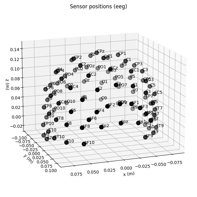
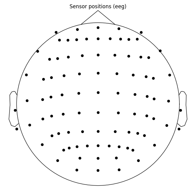
In the sample data, setting the digitized EEG montage was done prior to saving the Raw object to disk, so the sensor positions are already incorporated into the info attribute of the Raw object (see the documentation of the reading functions and set_montage() for details on how that works). Because of that, we can plot sensor locations directly from the Raw object using the plot_sensors() method, which provides similar functionality to montage.plot(). 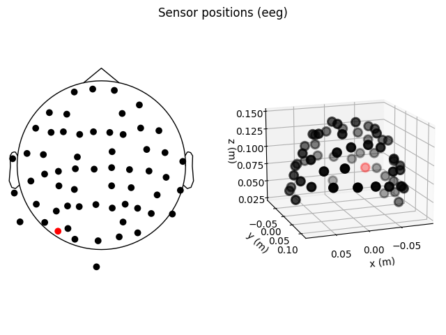plot_sensors() also allows channel selection by type, can color-code channels in various ways (by default, channels listed in raw.info['bads'] will be plotted in red), and allows drawing into an existing matplotlib axes object (so the channel positions can easily be made as a subplot in a multi-panel figure):

fig = plt.figure()
ax2d = fig.add_subplot(121)
ax3d = fig.add_subplot(122, projection='3d')
raw.plot_sensors(ch_type='eeg', axes=ax2d)
raw.plot_sensors(ch_type='eeg', axes=ax3d, kind='3d')
ax3d.view_init(azim=70, elev=15)

It’s probably evident from the 2D topomap above that there is some irregularity in the EEG sensor positions in the sample dataset — this is because the sensor positions in that dataset are digitizations of the sensor positions on an actual subject’s head, rather than idealized sensor positions based on a spherical head model. Depending on what system was used to digitize the electrode positions (e.g., a Polhemus Fastrak digitizer), you must use different montage reading functions (see Supported formats for digitized 3D locations). The resulting montage can then be added to Raw objects by passing it to the set_montage() method (just as we did above with the name of the idealized montage 'standard_1020'). Once loaded, locations can be plotted with plot() and saved with save(), like when working with a standard montage.

Note

When setting a montage with set_montage() the measurement info is updated in two places (the chs and dig entries are updated). See The Info data structure. dig may contain HPI, fiducial, or head shape points in addition to electrode locations.

Rendering sensor position with mayavi

It is also possible to render an image of a MEG sensor helmet in 3D, using mayavi instead of matplotlib, by calling the mne.viz.plot_alignment() function:

fig = mne.viz.plot_alignment(raw.info, trans=None, dig=False, eeg=False,
                             surfaces=[], meg=['helmet', 'sensors'],
                             coord_frame='meg')
mne.viz.set_3d_view(fig, azimuth=50, elevation=90, distance=0.5)

Out:

Getting helmet for system 306m

plot_alignment() requires an Info object, and can also render MRI surfaces of the scalp, skull, and brain (by passing keywords like 'head', 'outer_skull', or 'brain' to the surfaces parameter) making it useful for assessing coordinate frame transformations. For examples of various uses of plot_alignment(), see Plotting sensor layouts of EEG systems, Plotting EEG sensors on the scalp, and Plotting sensor layouts of MEG systems.

Working with layout files

As with montages, many layout files are included during MNE-Python installation, and are stored in the mne/channels/data/layouts folder:

layout_dir = os.path.join(os.path.dirname(mne.__file__),
                          'channels', 'data', 'layouts')
print('\nBUILT-IN LAYOUT FILES')
print('=====================')
print(sorted(os.listdir(layout_dir)))

Out:

BUILT-IN LAYOUT FILES
=====================
['CTF-275.lout', 'CTF151.lay', 'CTF275.lay', 'EEG1005.lay', 'EGI256.lout', 'KIT-125.lout', 'KIT-157.lout', 'KIT-160.lay', 'KIT-AD.lout', 'KIT-AS-2008.lout', 'KIT-UMD-3.lout', 'Neuromag_122.lout', 'Vectorview-all.lout', 'Vectorview-grad.lout', 'Vectorview-grad_norm.lout', 'Vectorview-mag.lout', 'biosemi.lay', 'magnesWH3600.lout']

You may have noticed that the file formats and filename extensions of the built-in layout and montage files vary considerably. This reflects different manufacturers’ conventions; to make loading easier the montage and layout loading functions in MNE-Python take the filename without its extension so you don’t have to keep track of which file format is used by which manufacturer.

To load a layout file, use the mne.channels.read_layout() function, and provide the filename without its file extension. You can then visualize the layout using its plot() method, or (equivalently) by passing it to mne.viz.plot_layout():

biosemi_layout = mne.channels.read_layout('biosemi')
biosemi_layout.plot()  # same result as: mne.viz.plot_layout(biosemi_layout)

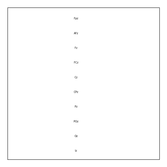
Similar to the picks argument for selecting channels from Raw objects, the plot() method of Layout objects also has a picks argument. However, because layouts only contain information about sensor name and location (not sensor type), the plot() method only allows picking channels by index (not by name or by type). Here we find the indices we want using numpy.where(); selection by name or type is possible via mne.pick_channels() or mne.pick_types().

midline = np.where([name.endswith('z') for name in biosemi_layout.names])[0]
biosemi_layout.plot(picks=midline)

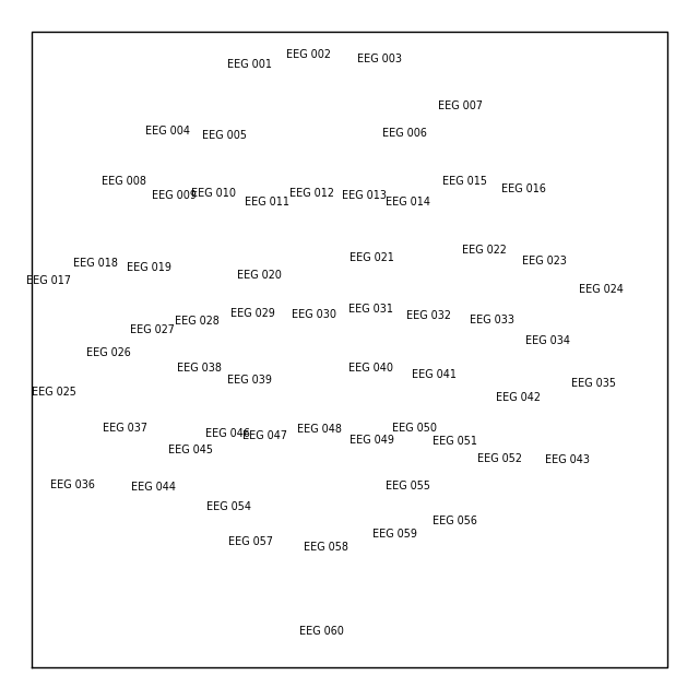
If you’re working with a Raw object that already has sensor positions incorporated, you can create a Layout object with either the mne.channels.make_eeg_layout() function or (equivalently) the mne.channels.find_layout() function.

layout_from_raw = mne.channels.make_eeg_layout(raw.info)
# same result as: mne.channels.find_layout(raw.info, ch_type='eeg')
layout_from_raw.plot()

Note

There is no corresponding make_meg_layout function because sensor locations are fixed in a MEG system (unlike in EEG, where the sensor caps deform to fit each subject’s head). Thus MEG layouts are consistent for a given system and you can simply load them with mne.channels.read_layout(), or use mne.channels.find_layout() with the ch_type parameter, as shown above for EEG.

All Layout objects have a save() method that allows writing layouts to disk, in either .lout or .lay format (which format gets written is inferred from the file extension you pass to the method’s fname parameter). The choice between .lout and .lay format only matters if you need to load the layout file in some other software (MNE-Python can read either format equally well).

Estimated memory usage: 492 MB