Make figures more publication ready¶

In this example, we take some MNE plots and make some changes to make a figure closer to publication-ready.

# Authors: Eric Larson <larson.eric.d@gmail.com>
#          Daniel McCloy <dan.mccloy@gmail.com>
#
# License: BSD (3-clause)

import os.path as op

import numpy as np
import matplotlib.pyplot as plt
from mpl_toolkits.axes_grid1 import make_axes_locatable, ImageGrid

import mne

Suppose we want a figure with an evoked plot on top, and the brain activation below, with the brain subplot slightly bigger than the evoked plot. Let’s start by loading some example data.

data_path = mne.datasets.sample.data_path()
subjects_dir = op.join(data_path, 'subjects')
fname_stc = op.join(data_path, 'MEG', 'sample', 'sample_audvis-meg-eeg-lh.stc')
fname_evoked = op.join(data_path, 'MEG', 'sample', 'sample_audvis-ave.fif')

evoked = mne.read_evokeds(fname_evoked, 'Left Auditory')
evoked.pick_types(meg='grad').apply_baseline((None, 0.))
max_t = evoked.get_peak()[1]

stc = mne.read_source_estimate(fname_stc)

Out:

Reading /home/circleci/mne_data/MNE-sample-data/MEG/sample/sample_audvis-ave.fif ...
    Read a total of 4 projection items:
        PCA-v1 (1 x 102) active
        PCA-v2 (1 x 102) active
        PCA-v3 (1 x 102) active
        Average EEG reference (1 x 60) active
    Found the data of interest:
        t =    -199.80 ...     499.49 ms (Left Auditory)
        0 CTF compensation matrices available
        nave = 55 - aspect type = 100
Projections have already been applied. Setting proj attribute to True.
No baseline correction applied
Removing projector <Projection | PCA-v1, active : True, n_channels : 102>
Removing projector <Projection | PCA-v2, active : True, n_channels : 102>
Removing projector <Projection | PCA-v3, active : True, n_channels : 102>
Removing projector <Projection | Average EEG reference, active : True, n_channels : 60>
Applying baseline correction (mode: mean)

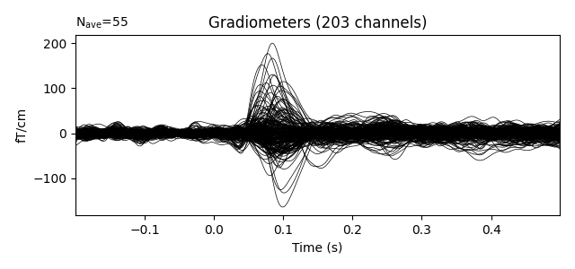
During interactive plotting, we might see figures like this:

evoked.plot()

stc.plot(views='lat', hemi='split', size=(800, 400), subject='sample',
         subjects_dir=subjects_dir, initial_time=max_t,
         time_viewer=False, show_traces=False)

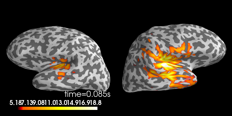
Out:

Using control points [ 5.17909658  6.18448887 18.83197989]

To make a publication-ready figure, first we’ll re-plot the brain on a white background, take a screenshot of it, and then crop out the white margins. While we’re at it, let’s change the colormap, set custom colormap limits and remove the default colorbar (so we can add a smaller, vertical one later):

colormap = 'viridis'
clim = dict(kind='value', lims=[4, 8, 12])

# Plot the STC, get the brain image, crop it:
brain = stc.plot(views='lat', hemi='split', size=(800, 400), subject='sample',
                 subjects_dir=subjects_dir, initial_time=max_t, background='w',
                 colorbar=False, clim=clim, colormap=colormap,
                 time_viewer=False, show_traces=False)
screenshot = brain.screenshot()
brain.close()

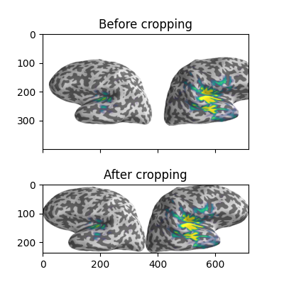
Now let’s crop out the white margins and the white gap between hemispheres. The screenshot has dimensions (h, w, 3), with the last axis being R, G, B values for each pixel, encoded as integers between 0 and 255. (255, 255, 255) encodes a white pixel, so we’ll detect any pixels that differ from that:

nonwhite_pix = (screenshot != 255).any(-1)
nonwhite_row = nonwhite_pix.any(1)
nonwhite_col = nonwhite_pix.any(0)
cropped_screenshot = screenshot[nonwhite_row][:, nonwhite_col]

# before/after results
fig = plt.figure(figsize=(4, 4))
axes = ImageGrid(fig, 111, nrows_ncols=(2, 1), axes_pad=0.5)
for ax, image, title in zip(axes, [screenshot, cropped_screenshot],
                            ['Before', 'After']):
    ax.imshow(image)
    ax.set_title('{} cropping'.format(title))

A lot of figure settings can be adjusted after the figure is created, but many can also be adjusted in advance by updating the rcParams dictionary. This is especially useful when your script generates several figures that you want to all have the same style:

# Tweak the figure style
plt.rcParams.update({
    'ytick.labelsize': 'small',
    'xtick.labelsize': 'small',
    'axes.labelsize': 'small',
    'axes.titlesize': 'medium',
    'grid.color': '0.75',
    'grid.linestyle': ':',
})

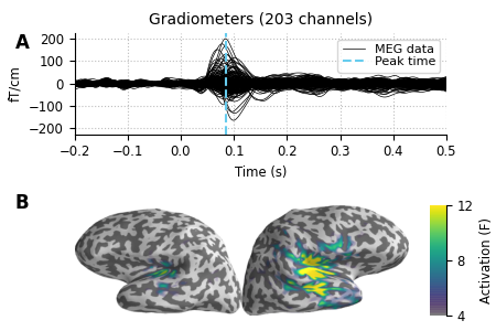
Now let’s create our custom figure. There are lots of ways to do this step. Here we’ll create the figure and the subplot axes in one step, specifying overall figure size, number and arrangement of subplots, and the ratio of subplot heights for each row using GridSpec keywords. Other approaches (using subplot2grid(), or adding each axes manually) are shown commented out, for reference.

# figsize unit is inches
fig, axes = plt.subplots(nrows=2, ncols=1, figsize=(4.5, 3.),
                         gridspec_kw=dict(height_ratios=[3, 4]))

# alternate way #1: using subplot2grid
# fig = plt.figure(figsize=(4.5, 3.))
# axes = [plt.subplot2grid((7, 1), (0, 0), rowspan=3),
#         plt.subplot2grid((7, 1), (3, 0), rowspan=4)]

# alternate way #2: using figure-relative coordinates
# fig = plt.figure(figsize=(4.5, 3.))
# axes = [fig.add_axes([0.125, 0.58, 0.775, 0.3]),  # left, bot., width, height
#         fig.add_axes([0.125, 0.11, 0.775, 0.4])]

# we'll put the evoked plot in the upper axes, and the brain below
evoked_idx = 0
brain_idx = 1

# plot the evoked in the desired subplot, and add a line at peak activation
evoked.plot(axes=axes[evoked_idx])
peak_line = axes[evoked_idx].axvline(max_t, color='#66CCEE', ls='--')
# custom legend
axes[evoked_idx].legend(
    [axes[evoked_idx].lines[0], peak_line], ['MEG data', 'Peak time'],
    frameon=True, columnspacing=0.1, labelspacing=0.1,
    fontsize=8, fancybox=True, handlelength=1.8)
# remove the "N_ave" annotation
axes[evoked_idx].texts = []
# Remove spines and add grid
axes[evoked_idx].grid(True)
axes[evoked_idx].set_axisbelow(True)
for key in ('top', 'right'):
    axes[evoked_idx].spines[key].set(visible=False)
# Tweak the ticks and limits
axes[evoked_idx].set(
    yticks=np.arange(-200, 201, 100), xticks=np.arange(-0.2, 0.51, 0.1))
axes[evoked_idx].set(
    ylim=[-225, 225], xlim=[-0.2, 0.5])

# now add the brain to the lower axes
axes[brain_idx].imshow(cropped_screenshot)
axes[brain_idx].axis('off')
# add a vertical colorbar with the same properties as the 3D one
divider = make_axes_locatable(axes[brain_idx])
cax = divider.append_axes('right', size='5%', pad=0.2)
cbar = mne.viz.plot_brain_colorbar(cax, clim, colormap, label='Activation (F)')

# tweak margins and spacing
fig.subplots_adjust(
    left=0.15, right=0.9, bottom=0.01, top=0.9, wspace=0.1, hspace=0.5)

# add subplot labels
for ax, label in zip(axes, 'AB'):
    ax.text(0.03, ax.get_position().ymax, label, transform=fig.transFigure,
            fontsize=12, fontweight='bold', va='top', ha='left')