Note
Click here to download the full example code
Head model and forward computation
The aim of this tutorial is to be a getting started for forward computation.
For more extensive details and presentation of the general concepts for forward modeling, see The forward solution.
import os.path as op
import mne
from mne.datasets import sample
data_path = sample.data_path()

# the raw file containing the channel location + types
raw_fname = data_path + '/MEG/sample/sample_audvis_raw.fif'
# The paths to Freesurfer reconstructions
subjects_dir = data_path + '/subjects'
subject = 'sample'
Computing the forward operator
To compute a forward operator we need:
a
-trans.fiffile that contains the coregistration info.a source space
the BEM surfaces
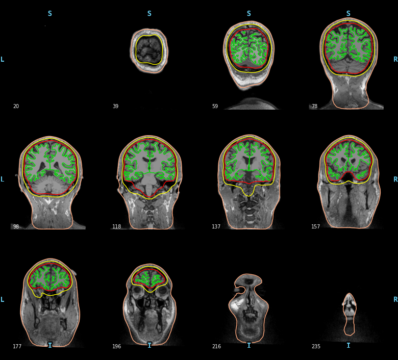
Compute and visualize BEM surfaces
The BEM surfaces are the triangulations of the interfaces between different tissues needed for forward computation. These surfaces are for example the inner skull surface, the outer skull surface and the outer skin surface, a.k.a. scalp surface.
Computing the BEM surfaces requires FreeSurfer and makes use of
the command-line tools mne watershed_bem or mne flash_bem, or
the related functions mne.bem.make_watershed_bem() or
mne.bem.make_flash_bem().
Here we’ll assume it’s already computed. It takes a few minutes per subject.
For EEG we use 3 layers (inner skull, outer skull, and skin) while for MEG 1 layer (inner skull) is enough.
Let’s look at these surfaces. The function mne.viz.plot_bem()
assumes that you have the bem folder of your subject’s FreeSurfer
reconstruction, containing the necessary surface files.
mne.viz.plot_bem(subject=subject, subjects_dir=subjects_dir,
                 brain_surfaces='white', orientation='coronal')
Out:
Using surface: /home/circleci/mne_data/MNE-sample-data/subjects/sample/bem/inner_skull.surf
Using surface: /home/circleci/mne_data/MNE-sample-data/subjects/sample/bem/outer_skull.surf
Using surface: /home/circleci/mne_data/MNE-sample-data/subjects/sample/bem/outer_skin.surf
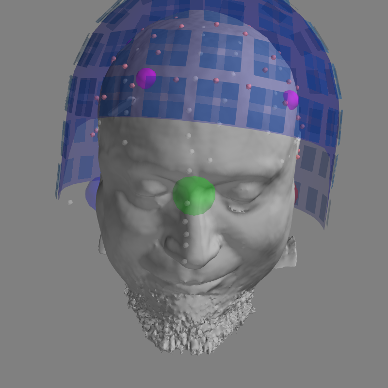
Visualizing the coregistration
The coregistration is the operation that allows to position the head and the
sensors in a common coordinate system. In the MNE software the transformation
to align the head and the sensors in stored in a so-called trans file.
It is a FIF file that ends with -trans.fif. It can be obtained with
mne.gui.coregistration() (or its convenient command line
equivalent mne coreg), or mrilab if you’re using a Neuromag
system.
Here we assume the coregistration is done, so we just visually check the alignment with the following code.
# The transformation file obtained by coregistration
trans = data_path + '/MEG/sample/sample_audvis_raw-trans.fif'

info = mne.io.read_info(raw_fname)
# Here we look at the dense head, which isn't used for BEM computations but
# is useful for coregistration.
mne.viz.plot_alignment(info, trans, subject=subject, dig=True,
                       meg=['helmet', 'sensors'], subjects_dir=subjects_dir,
                       surfaces='head-dense')
Out:
    Read a total of 3 projection items:
        PCA-v1 (1 x 10²)  idle
        PCA-v2 (1 x 10²)  idle
        PCA-v3 (1 x 10²)  idle
Using lh.seghead for head surface.
Getting helmet for system 306m
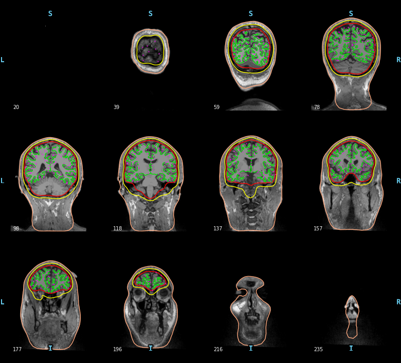
Compute Source Space
The source space defines the position and orientation of the candidate source locations. There are two types of source spaces:
surface-based source space when the candidates are confined to a surface.
volumetric or discrete source space when the candidates are discrete, arbitrarily located source points bounded by the surface.
Surface-based source space is computed using
mne.setup_source_space(), while volumetric source space is computed
using mne.setup_volume_source_space().
We will now compute a surface-based source space with an 'oct4'
resolution. See Setting up the source space for details on source space
definition and spacing parameter.
Warning
'oct4' is used here just for speed, for real analyses the recommended
spacing is 'oct6'.
src = mne.setup_source_space(subject, spacing='oct4', add_dist='patch',
                             subjects_dir=subjects_dir)
print(src)
Out:
Setting up the source space with the following parameters:

SUBJECTS_DIR = /home/circleci/mne_data/MNE-sample-data/subjects
Subject      = sample
Surface      = white
Octahedron subdivision grade 4

>>> 1. Creating the source space...

Doing the octahedral vertex picking...
Loading /home/circleci/mne_data/MNE-sample-data/subjects/sample/surf/lh.white...
Mapping lh sample -> oct (4) ...
    Triangle neighbors and vertex normals...
Loading geometry from /home/circleci/mne_data/MNE-sample-data/subjects/sample/surf/lh.sphere...
Setting up the triangulation for the decimated surface...
loaded lh.white 258/155407 selected to source space (oct = 4)

Loading /home/circleci/mne_data/MNE-sample-data/subjects/sample/surf/rh.white...
Mapping rh sample -> oct (4) ...
    Triangle neighbors and vertex normals...
Loading geometry from /home/circleci/mne_data/MNE-sample-data/subjects/sample/surf/rh.sphere...
Setting up the triangulation for the decimated surface...
loaded rh.white 258/156866 selected to source space (oct = 4)

Calculating patch information (limit=0.0 mm)...
    Computing patch statistics...
    Patch information added...
    Computing patch statistics...
    Patch information added...
You are now one step closer to computing the gain matrix
<SourceSpaces: [<surface (lh), n_vertices=155407, n_used=258>, <surface (rh), n_vertices=156866, n_used=258>] MRI (surface RAS) coords, subject 'sample', ~28.7 MB>
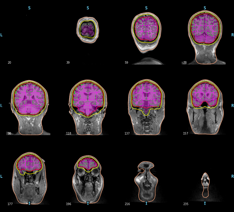
The surface based source space src contains two parts, one for the left
hemisphere (258 locations) and one for the right hemisphere (258
locations). Sources can be visualized on top of the BEM surfaces in purple.
mne.viz.plot_bem(subject=subject, subjects_dir=subjects_dir,
                 brain_surfaces='white', src=src, orientation='coronal')
Out:
Using surface: /home/circleci/mne_data/MNE-sample-data/subjects/sample/bem/inner_skull.surf
Using surface: /home/circleci/mne_data/MNE-sample-data/subjects/sample/bem/outer_skull.surf
Using surface: /home/circleci/mne_data/MNE-sample-data/subjects/sample/bem/outer_skin.surf
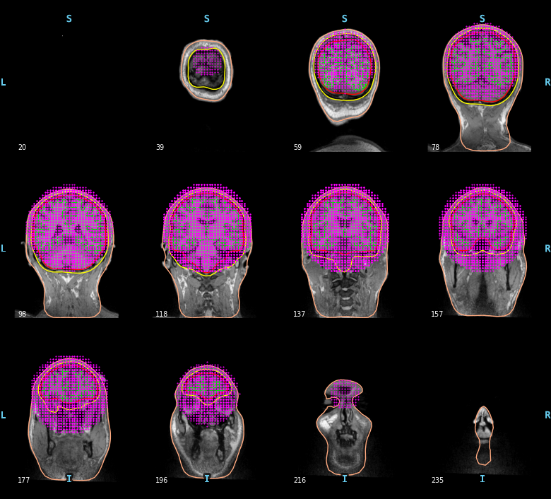
To compute a volume based source space defined with a grid of candidate dipoles inside a sphere of radius 90mm centered at (0.0, 0.0, 40.0) mm you can use the following code. Obviously here, the sphere is not perfect. It is not restricted to the brain and it can miss some parts of the cortex.
sphere = (0.0, 0.0, 0.04, 0.09)
vol_src = mne.setup_volume_source_space(subject, subjects_dir=subjects_dir,
                                        sphere=sphere, sphere_units='m')
print(vol_src)

mne.viz.plot_bem(subject=subject, subjects_dir=subjects_dir,
                 brain_surfaces='white', src=vol_src, orientation='coronal')
Out:
Sphere                : origin at (0.0 0.0 40.0) mm
              radius  : 90.0 mm
grid                  : 5.0 mm
mindist               : 5.0 mm
MRI volume            : /home/circleci/mne_data/MNE-sample-data/subjects/sample/mri/T1.mgz

Reading /home/circleci/mne_data/MNE-sample-data/subjects/sample/mri/T1.mgz...

Setting up the sphere...
Surface CM = (   0.0    0.0   40.0) mm
Surface fits inside a sphere with radius   90.0 mm
Surface extent:
    x =  -90.0 ...   90.0 mm
    y =  -90.0 ...   90.0 mm
    z =  -50.0 ...  130.0 mm
Grid extent:
    x =  -95.0 ...   95.0 mm
    y =  -95.0 ...   95.0 mm
    z =  -50.0 ...  135.0 mm
57798 sources before omitting any.
24365 sources after omitting infeasible sources not within 0.0 - 90.0 mm.
20377 sources remaining after excluding the sources outside the surface and less than    5.0 mm inside.
Adjusting the neighborhood info.
Source space : MRI voxel -> MRI (surface RAS)
     0.005000  0.000000  0.000000     -95.00 mm
     0.000000  0.005000  0.000000     -95.00 mm
     0.000000  0.000000  0.005000     -50.00 mm
     0.000000  0.000000  0.000000       1.00
MRI volume : MRI voxel -> MRI (surface RAS)
    -0.001000  0.000000  0.000000     128.00 mm
     0.000000  0.000000  0.001000    -128.00 mm
     0.000000 -0.001000  0.000000     128.00 mm
     0.000000  0.000000  0.000000       1.00
MRI volume : MRI (surface RAS) -> RAS (non-zero origin)
     1.000000 -0.000000 -0.000000      -5.27 mm
    -0.000000  1.000000 -0.000000       9.04 mm
    -0.000000  0.000000  1.000000     -27.29 mm
     0.000000  0.000000  0.000000       1.00
Setting up volume interpolation ...
    22994400/16777216 nonzero values for the whole brain
[done]
<SourceSpaces: [<volume, shape=(39, 39, 38), n_used=20377>] MRI (surface RAS) coords, subject 'sample', ~78.7 MB>
Using surface: /home/circleci/mne_data/MNE-sample-data/subjects/sample/bem/inner_skull.surf
Using surface: /home/circleci/mne_data/MNE-sample-data/subjects/sample/bem/outer_skull.surf
Using surface: /home/circleci/mne_data/MNE-sample-data/subjects/sample/bem/outer_skin.surf
To compute a volume based source space defined with a grid of candidate dipoles inside the brain (requires the BEM surfaces) you can use the following.
surface = op.join(subjects_dir, subject, 'bem', 'inner_skull.surf')
vol_src = mne.setup_volume_source_space(subject, subjects_dir=subjects_dir,
                                        surface=surface)
print(vol_src)

mne.viz.plot_bem(subject=subject, subjects_dir=subjects_dir,
                 brain_surfaces='white', src=vol_src, orientation='coronal')
Out:
Boundary surface file : /home/circleci/mne_data/MNE-sample-data/subjects/sample/bem/inner_skull.surf
grid                  : 5.0 mm
mindist               : 5.0 mm
MRI volume            : /home/circleci/mne_data/MNE-sample-data/subjects/sample/mri/T1.mgz

Reading /home/circleci/mne_data/MNE-sample-data/subjects/sample/mri/T1.mgz...

Loaded bounding surface from /home/circleci/mne_data/MNE-sample-data/subjects/sample/bem/inner_skull.surf (2562 nodes)
Surface CM = (   0.7  -10.0   44.3) mm
Surface fits inside a sphere with radius   91.8 mm
Surface extent:
    x =  -66.7 ...   68.8 mm
    y =  -88.0 ...   79.0 mm
    z =  -44.5 ...  105.8 mm
Grid extent:
    x =  -70.0 ...   70.0 mm
    y =  -90.0 ...   80.0 mm
    z =  -45.0 ...  110.0 mm
32480 sources before omitting any.
22941 sources after omitting infeasible sources not within 0.0 - 91.8 mm.
Source spaces are in MRI coordinates.
Checking that the sources are inside the surface and at least    5.0 mm away (will take a few...)
    Skipping interior check for 2787 sources that fit inside a sphere of radius   43.6 mm
    Skipping solid angle check for 9357 points using Qhull
    10203 source space points omitted because they are outside the inner skull surface.
    2362 source space points omitted because of the    5.0-mm distance limit.
10376 sources remaining after excluding the sources outside the surface and less than    5.0 mm inside.
Adjusting the neighborhood info.
Source space : MRI voxel -> MRI (surface RAS)
     0.005000  0.000000  0.000000     -70.00 mm
     0.000000  0.005000  0.000000     -90.00 mm
     0.000000  0.000000  0.005000     -45.00 mm
     0.000000  0.000000  0.000000       1.00
MRI volume : MRI voxel -> MRI (surface RAS)
    -0.001000  0.000000  0.000000     128.00 mm
     0.000000  0.000000  0.001000    -128.00 mm
     0.000000 -0.001000  0.000000     128.00 mm
     0.000000  0.000000  0.000000       1.00
MRI volume : MRI (surface RAS) -> RAS (non-zero origin)
     1.000000 -0.000000 -0.000000      -5.27 mm
    -0.000000  1.000000 -0.000000       9.04 mm
    -0.000000  0.000000  1.000000     -27.29 mm
     0.000000  0.000000  0.000000       1.00
Setting up volume interpolation ...
    12329000/16777216 nonzero values for the whole brain
[done]
<SourceSpaces: [<volume, shape=(29, 35, 32), n_used=10376>] MRI (surface RAS) coords, subject 'sample', ~72.3 MB>
Using surface: /home/circleci/mne_data/MNE-sample-data/subjects/sample/bem/inner_skull.surf
Using surface: /home/circleci/mne_data/MNE-sample-data/subjects/sample/bem/outer_skull.surf
Using surface: /home/circleci/mne_data/MNE-sample-data/subjects/sample/bem/outer_skin.surf
Note
Some sources may appear to be outside the BEM inner skull contour.
This is because the slices are decimated for plotting here.
Each slice in the figure actually represents several MRI slices,
but only the MRI voxels and BEM boundaries for a single (midpoint
of the given slice range) slice are shown, whereas the source space
points plotted on that midpoint slice consist of all points
for which that slice (out of all slices shown) was the closest.
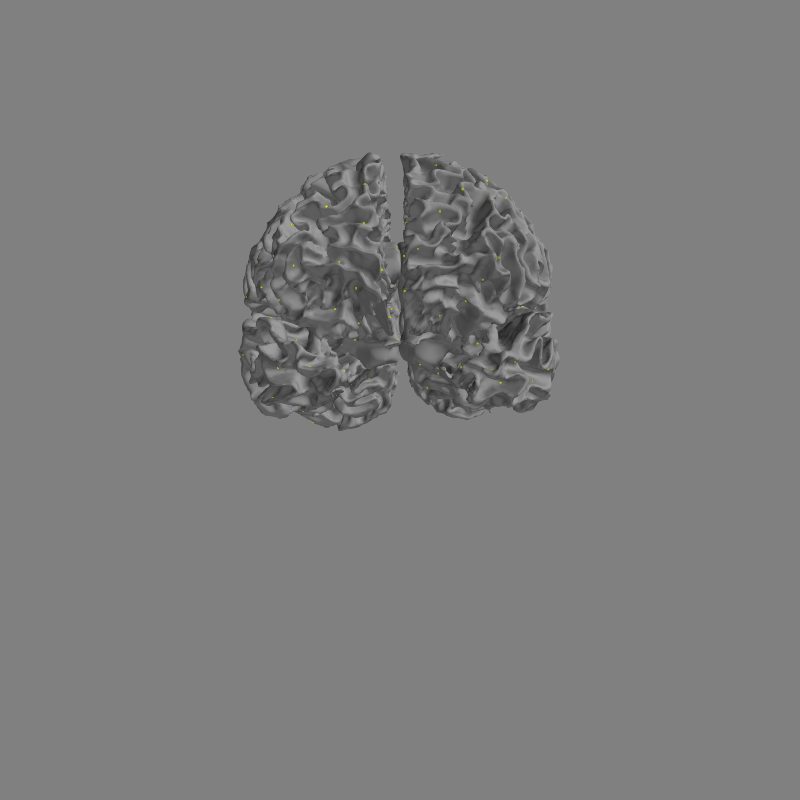
Now let’s see how to view all sources in 3D.
fig = mne.viz.plot_alignment(subject=subject, subjects_dir=subjects_dir,
                             surfaces='white', coord_frame='head',
                             src=src)
mne.viz.set_3d_view(fig, azimuth=173.78, elevation=101.75,
                    distance=0.30, focalpoint=(-0.03, -0.01, 0.03))
Compute forward solution
We can now compute the forward solution.
To reduce computation we’ll just compute a single layer BEM (just inner
skull) that can then be used for MEG (not EEG).
We specify if we want a one-layer or a three-layer BEM using the
conductivity parameter.
The BEM solution requires a BEM model which describes the geometry
of the head the conductivities of the different tissues.
conductivity = (0.3,)  # for single layer
# conductivity = (0.3, 0.006, 0.3)  # for three layers
model = mne.make_bem_model(subject='sample', ico=4,
                           conductivity=conductivity,
                           subjects_dir=subjects_dir)
bem = mne.make_bem_solution(model)
Out:
Creating the BEM geometry...
Going from 4th to 4th subdivision of an icosahedron (n_tri: 5120 -> 5120)
inner skull CM is   0.67 -10.01  44.26 mm
Surfaces passed the basic topology checks.
Complete.

Approximation method : Linear collocation

Homogeneous model surface loaded.
Computing the linear collocation solution...
    Matrix coefficients...
        inner skull (2562) -> inner skull (2562) ...
    Inverting the coefficient matrix...
Solution ready.
BEM geometry computations complete.
Note that the BEM does not involve any use of the trans file. The BEM only depends on the head geometry and conductivities. It is therefore independent from the MEG data and the head position.
Let’s now compute the forward operator, commonly referred to as the
gain or leadfield matrix.
See mne.make_forward_solution() for details on the meaning of each
parameter.
Out:
Source space          : <SourceSpaces: [<surface (lh), n_vertices=155407, n_used=258>, <surface (rh), n_vertices=156866, n_used=258>] MRI (surface RAS) coords, subject 'sample', ~28.7 MB>
MRI -> head transform : /home/circleci/mne_data/MNE-sample-data/MEG/sample/sample_audvis_raw-trans.fif
Measurement data      : sample_audvis_raw.fif
Conductor model   : instance of ConductorModel
Accurate field computations
Do computations in head coordinates
Free source orientations

Read 2 source spaces a total of 516 active source locations

Coordinate transformation: MRI (surface RAS) -> head
     0.999310  0.009985 -0.035787      -3.17 mm
     0.012759  0.812405  0.582954       6.86 mm
     0.034894 -0.583008  0.811716      28.88 mm
     0.000000  0.000000  0.000000       1.00

Read 306 MEG channels from info
99 coil definitions read
Coordinate transformation: MEG device -> head
     0.991420 -0.039936 -0.124467      -6.13 mm
     0.060661  0.984012  0.167456       0.06 mm
     0.115790 -0.173570  0.977991      64.74 mm
     0.000000  0.000000  0.000000       1.00
MEG coil definitions created in head coordinates.
Source spaces are now in head coordinates.

Employing the head->MRI coordinate transform with the BEM model.
BEM model instance of ConductorModel is now set up

Source spaces are in head coordinates.
Checking that the sources are inside the surface and at least    5.0 mm away (will take a few...)
    Skipping interior check for 54 sources that fit inside a sphere of radius   43.6 mm
    Skipping solid angle check for 0 points using Qhull
    23 source space point omitted because of the    5.0-mm distance limit.
    Computing patch statistics...
    Patch information added...
    Skipping interior check for 51 sources that fit inside a sphere of radius   43.6 mm
    Skipping solid angle check for 0 points using Qhull
    19 source space point omitted because of the    5.0-mm distance limit.
    Computing patch statistics...
    Patch information added...

Setting up compensation data...
    No compensation set. Nothing more to do.

Composing the field computation matrix...
Computing MEG at 474 source locations (free orientations)...

Finished.
<Forward | MEG channels: 306 | EEG channels: 0 | Source space: Surface with 474 vertices | Source orientation: Free>
Warning
Forward computation can remove vertices that are too close to (or outside)
the inner skull surface. For example, here we have gone from 516 to 474
vertices in use. For many functions, such as
mne.compute_source_morph(), it is important to pass fwd['src']
or inv['src'] so that this removal is adequately accounted for.
Out:
Before: <SourceSpaces: [<surface (lh), n_vertices=155407, n_used=258>, <surface (rh), n_vertices=156866, n_used=258>] MRI (surface RAS) coords, subject 'sample', ~28.7 MB>
After:  <SourceSpaces: [<surface (lh), n_vertices=155407, n_used=235>, <surface (rh), n_vertices=156866, n_used=239>] head coords, subject 'sample', ~28.7 MB>
We can explore the content of fwd to access the numpy array that contains
the gain matrix.
leadfield = fwd['sol']['data']
print("Leadfield size : %d sensors x %d dipoles" % leadfield.shape)
Out:
Leadfield size : 306 sensors x 1422 dipoles
To extract the numpy array containing the forward operator corresponding to
the source space fwd['src'] with cortical orientation constraint
we can use the following:
fwd_fixed = mne.convert_forward_solution(fwd, surf_ori=True, force_fixed=True,
                                         use_cps=True)
leadfield = fwd_fixed['sol']['data']
print("Leadfield size : %d sensors x %d dipoles" % leadfield.shape)
Out:
    Average patch normals will be employed in the rotation to the local surface coordinates....
    Converting to surface-based source orientations...
    [done]
Leadfield size : 306 sensors x 474 dipoles
This is equivalent to the following code that explicitly applies the forward operator to a source estimate composed of the identity operator (which we omit here because it uses a lot of memory):
>>> import numpy as np
>>> n_dipoles = leadfield.shape[1]
>>> vertices = [src_hemi['vertno'] for src_hemi in fwd_fixed['src']]
>>> stc = mne.SourceEstimate(1e-9 * np.eye(n_dipoles), vertices)
>>> leadfield = mne.apply_forward(fwd_fixed, stc, info).data / 1e-9
To save to disk a forward solution you can use
mne.write_forward_solution() and to read it back from disk
mne.read_forward_solution(). Don’t forget that FIF files containing
forward solution should end with -fwd.fif.
To get a fixed-orientation forward solution, use
mne.convert_forward_solution() to convert the free-orientation
solution to (surface-oriented) fixed orientation.
Exercise
By looking at Display sensitivity maps for EEG and MEG sensors plot the sensitivity maps for EEG and compare it with the MEG, can you justify the claims that:
MEG is not sensitive to radial sources
EEG is more sensitive to deep sources
How will the MEG sensitivity maps and histograms change if you use a free instead if a fixed/surface oriented orientation?
Try this changing the mode parameter in mne.sensitivity_map()
accordingly. Why don’t we see any dipoles on the gyri?
Total running time of the script: ( 1 minutes 7.703 seconds)
Estimated memory usage: 378 MB