01. Detect HFOs in Simulated Dataset

MNE-HFO currently depends on the data structures defined by MNE-Python. Namely the mne.io.Raw object.

In this example, we use MNE-HFO to simulate raw data and detect HFOs. Specifically, we will follow these steps:

1. Create some simulated data and artificially simulate a few HFOs

2. Run a few mne_hfo.base.Detector instances to detect HFOs

3. Format the detected HFOs as a pandas.DataFrame

4. Write to disk and read it in again.

# Authors: Adam Li <adam2392@gmail.com>
#

We are importing everything we need for this example:

import numpy as np
from mne import create_info
from mne.io import RawArray

from mne_hfo import (RMSDetector, compute_chs_hfo_rates)
from mne_hfo.simulate import simulate_hfo

Simulate the data

First, we need some data to work with. We will use a fake dataset that we simulate.

In this example, we will simulate sinusoidal data that has an artificial HFO added at two points with 9 cycles each.

# simulate the testing dataset
freqs = [2.5, 6.0, 10.0, 16.0, 32.5, 67.5, 165.0,
         250.0, 425.0, 500.0, 800.0, 1500.0]

# sampling frequency
sfreq = 2000

# number of seconds to simulate
n = sfreq * 10
data = np.zeros(n)

# generate some sinusoidal data at specified frequencies
x = np.arange(n)
for freq in freqs:
    # freq_amp = basic_amp / freq
    y = np.sin(2 * np.pi * freq * x / sfreq)
    data += y

# We have dummy data now inject 2 HFOs
freq = 250
numcycles = 9
sim = simulate_hfo(sfreq, freq, numcycles)[0]
ev_start = sfreq
data[ev_start: ev_start + len(sim)] += sim * 10

sim = simulate_hfo(sfreq, freq, numcycles)[0]
ev_start = 7 * sfreq
data[ev_start: ev_start + len(sim)] += sim * 10

# convert the data into mne-python
# note: the channel names are made up and the channel types are just
# set to 'seeg' for the sake of the example
ch_names = ['A1']
info = create_info(sfreq=sfreq, ch_names=ch_names, ch_types='seeg')
raw = RawArray(data=data[np.newaxis, :], info=info)

Creating RawArray with float64 data, n_channels=1, n_times=20000
    Range : 0 ... 19999 =      0.000 ...     9.999 secs
Ready.

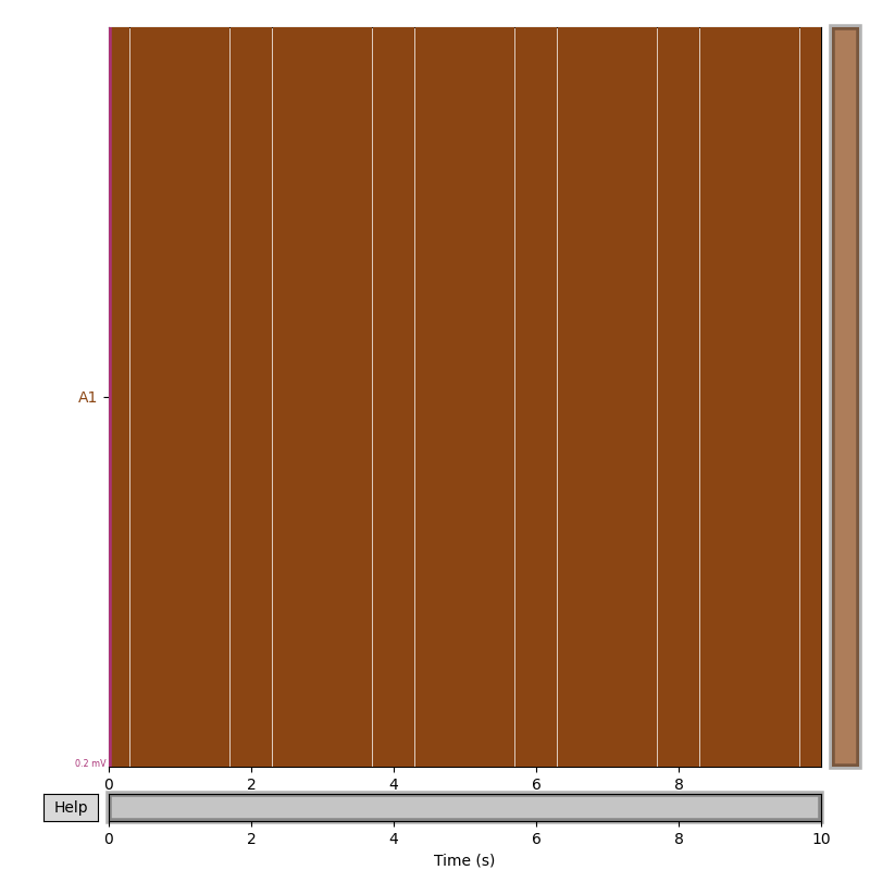
Let’s plot the data and see what it looks like

raw.plot()

Using matplotlib as 2D backend.

Detect HFOs

All detectors inherit from the base class mne_hfo.base.Detector, which inherits from the sklearn.base.BaseEstimator class. To run any estimator, one instantiates it along with the hyper-parameters, and then calls the fit function. Afterwards, detected HFOs are available in the various data structures. The recommended usage is the DataFrame, which is accessible via the mne_hfo.base.Detector.to_data_frame property.

kwargs = {
    'threshold': 3,  # threshold for "significance"
    'win_size': 100,  # window size in samples
    'overlap': 0.25  # overlap in percentage relative to the window size
}
detector = RMSDetector(**kwargs)

# run detector
detector.fit(X=raw)

# show all the HFO annotations
print(detector.hfo_annotations)

# get the dataframe of the Annotations
df = detector.to_data_frame()
print(df.head())

  0%|          | 0/1 [00:00<?, ?it/s]
100%|██████████| 1/1 [00:00<00:00, 53.78it/s]
<Annotations | 2 segments, channel-specific: hfo (2)>
                onset  ...  ch_names
0 1970-01-01 00:00:01  ...     (A1,)
1 1970-01-01 00:00:07  ...     (A1,)

[2 rows x 4 columns]

Convert HFO events to annotations

Detectors output HFO events detected as a DataFrame fashioned after the *_events.tsv files in BIDS-iEEG. Instead, HFO events are indeed Derivatives of the Raw data, that are estimated/detected using mne-hfo. The correct way to store them is in terms of an *_annotations.tsv, according to the BIDS-Derivatives specification.

# convert to annotation df
annot_df = detector.to_data_frame(format='bids')
print(annot_df.head())

  onset  ...   sfreq
0   1.0  ...  2000.0
1   7.0  ...  2000.0

[2 rows x 6 columns]
   onset  ...   sfreq
0    1.0  ...  2000.0
1    7.0  ...  2000.0

[2 rows x 6 columns]

compute HFO rate as HFOs per second

ch_rates = compute_chs_hfo_rates(annot_df=annot_df, rate='s')
print(ch_rates)

Beginning timestamp: 2023-09-21 21:30:27.613463+00:00
Got end timestamp of: 2023-09-21 21:30:34.613463+00:00
Found HFO rate per s for A1 as 0.2857142857142857
defaultdict(<class 'list'>, {'A1': 0.2857142857142857})

Estimated memory usage: 181 MB