Repairing artifacts with ICA automatically using ICLabel Model

This tutorial covers automatically repairing signals using ICA with the ICLabel model [1], which originates in EEGLab. For conceptual background on ICA, see this scikit-learn tutorial. For a basic understanding of how to use ICA to remove artifacts, see the tutorial in MNE-Python.

We begin as always by importing the necessary Python modules and loading some example data. Because ICA can be computationally intense, we’ll also crop the data to 60 seconds; and to save ourselves from repeatedly typing mne.preprocessing we’ll directly import a few functions and classes from that submodule.

import os

import mne
from mne.preprocessing import ICA

from mne_icalabel import label_components

sample_data_folder = mne.datasets.sample.data_path()
sample_data_raw_file = os.path.join(
    sample_data_folder, "MEG", "sample", "sample_audvis_filt-0-40_raw.fif"
)
raw = mne.io.read_raw_fif(sample_data_raw_file)

# Here we'll crop to 60 seconds and drop gradiometer channels for speed
raw.crop(tmax=60.0).pick_types(meg="mag", eeg=True, stim=True, eog=True)
raw.load_data()

Opening raw data file /home/scheltie/mne_data/MNE-sample-data/MEG/sample/sample_audvis_filt-0-40_raw.fif...
    Read a total of 4 projection items:
        PCA-v1 (1 x 102)  idle
        PCA-v2 (1 x 102)  idle
        PCA-v3 (1 x 102)  idle
        Average EEG reference (1 x 60)  idle
    Range : 6450 ... 48149 =     42.956 ...   320.665 secs
Ready.
NOTE: pick_types() is a legacy function. New code should use inst.pick(...).
Reading 0 ... 9009  =      0.000 ...    59.999 secs...

Measurement date	December 03, 2002 19:01:10 GMT
Experimenter	Unknown
Participant	Unknown
Digitized points	146 points
Good channels	102 Magnetometers, 9 Stimulus, 59 EEG, 1 EOG
Bad channels	None
EOG channels	EOG 061
ECG channels	Not available
Sampling frequency	150.15 Hz
Highpass	0.10 Hz
Lowpass	40.00 Hz
Projections	PCA-v1 : off PCA-v2 : off PCA-v3 : off Average EEG reference : off
Filenames	sample_audvis_filt-0-40_raw.fif
Duration	00:00:60 (HH:MM:SS)

Note

Before applying ICA (or any artifact repair strategy), be sure to observe the artifacts in your data to make sure you choose the right repair tool. Sometimes the right tool is no tool at all — if the artifacts are small enough you may not even need to repair them to get good analysis results. See Overview of artifact detection for guidance on detecting and visualizing various types of artifact.

# Example: EOG and ECG artifact repair
# ^^^^^^^^^^^^^^^^^^^^^^^^^^^^^^^^^^^^
#
# Visualizing the artifacts
# ~~~~~~~~~~~~~~~~~~~~~~~~~
#
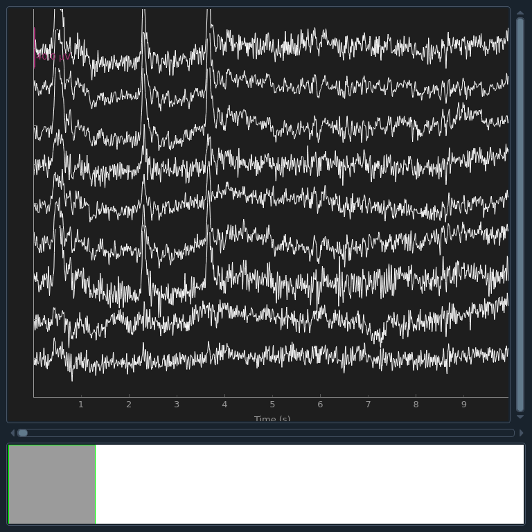
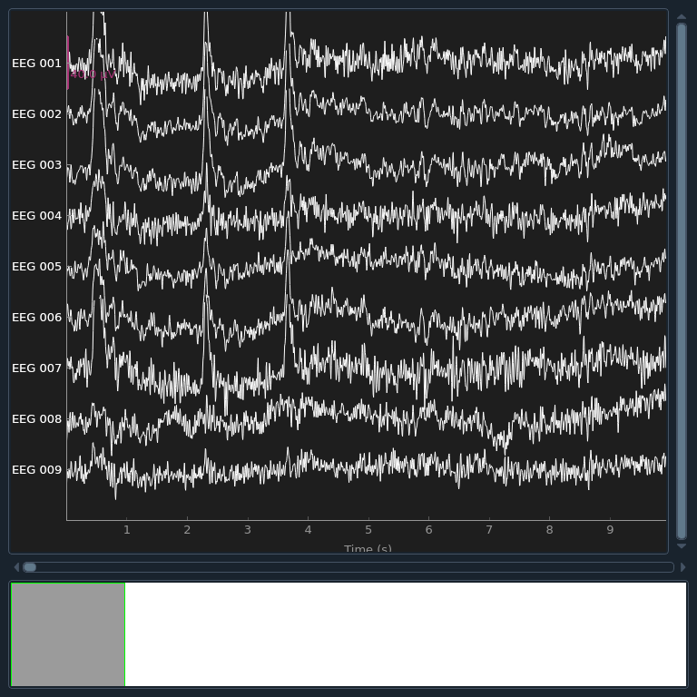
# Let's begin by visualizing the artifacts that we want to repair. In this
# dataset they are big enough to see easily in the raw data:

# Note: for this example, we are using ICLabel which has only
# been validated and works for EEG systems with less than 32 electrodes.
raw = raw.pick_types(eeg=True, eog=True, ecg=True, emg=True)

# pick some channels that clearly show heartbeats and blinks
regexp = r"(EEG 00.)"
artifact_picks = mne.pick_channels_regexp(raw.ch_names, regexp=regexp)
raw.plot(order=artifact_picks, n_channels=len(artifact_picks), show_scrollbars=False)

NOTE: pick_types() is a legacy function. New code should use inst.pick(...).
Removing projector <Projection | PCA-v1, active : False, n_channels : 102>
Removing projector <Projection | PCA-v2, active : False, n_channels : 102>
Removing projector <Projection | PCA-v3, active : False, n_channels : 102>

Filtering to remove slow drifts

Before we run the ICA, an important step is filtering the data to remove low-frequency drifts, which can negatively affect the quality of the ICA fit. The slow drifts are problematic because they reduce the independence of the assumed-to-be-independent sources (e.g., during a slow upward drift, the neural, heartbeat, blink, and other muscular sources will all tend to have higher values), making it harder for the algorithm to find an accurate solution. A high-pass filter with 1 Hz cutoff frequency is recommended. However, because filtering is a linear operation, the ICA solution found from the filtered signal can be applied to the unfiltered signal (see [2] for more information), so we’ll keep a copy of the unfiltered Raw object around so we can apply the ICA solution to it later.

filt_raw = raw.copy().filter(l_freq=1.0, h_freq=None)

Filtering raw data in 1 contiguous segment
Setting up high-pass filter at 1 Hz

FIR filter parameters
---------------------
Designing a one-pass, zero-phase, non-causal highpass filter:
- Windowed time-domain design (firwin) method
- Hamming window with 0.0194 passband ripple and 53 dB stopband attenuation
- Lower passband edge: 1.00
- Lower transition bandwidth: 1.00 Hz (-6 dB cutoff frequency: 0.50 Hz)
- Filter length: 497 samples (3.310 s)

[Parallel(n_jobs=1)]: Done  17 tasks      | elapsed:    0.0s

Fitting and plotting the ICA solution

Ignoring the time domain

The ICA algorithms implemented in MNE-Python find patterns across channels, but ignore the time domain. This means you can compute ICA on discontinuous Epochs or Evoked objects (not just continuous Raw objects), or only use every Nth sample by passing the decim parameter to ICA.fit().

Note

Epochs used for fitting ICA should not be baseline-corrected. Because cleaning the data via ICA may introduce DC offsets, we suggest to baseline correct your data after cleaning (and not before), should you require baseline correction.

Now we’re ready to set up and fit the ICA. Since we know (from observing our raw data) that the EOG and ECG artifacts are fairly strong, we would expect those artifacts to be captured in the first few dimensions of the PCA decomposition that happens before the ICA. Therefore, we probably don’t need a huge number of components to do a good job of isolating our artifacts (though it is usually preferable to include more components for a more accurate solution). As a first guess, we’ll run ICA with n_components=15 (use only the first 15 PCA components to compute the ICA decomposition) — a very small number given that our data has over 300 channels, but with the advantage that it will run quickly and we will able to tell easily whether it worked or not (because we already know what the EOG / ECG artifacts should look like).

ICA fitting is not deterministic (e.g., the components may get a sign flip on different runs, or may not always be returned in the same order), so we’ll also specify a random seed so that we get identical results each time this tutorial is built by our web servers.

ica = ICA(n_components=15, max_iter="auto", random_state=97)
ica.fit(filt_raw)
ica

Fitting ICA to data using 59 channels (please be patient, this may take a while)
Selecting by number: 15 components
Fitting ICA took 0.4s.

Method	fastica
Fit	92 iterations on raw data (9010 samples)
ICA components	15
Available PCA components	59
Channel types	eeg
ICA components marked for exclusion	—

Some optional parameters that we could have passed to the fit method include decim (to use only every Nth sample in computing the ICs, which can yield a considerable speed-up) and reject (for providing a rejection dictionary for maximum acceptable peak-to-peak amplitudes for each channel type, just like we used when creating epoched data in the Overview of MEG/EEG analysis with MNE-Python tutorial).

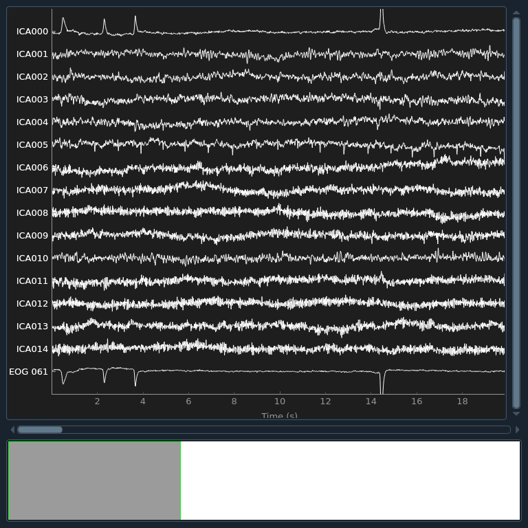
Now we can examine the ICs to see what they captured. plot_sources will show the time series of the ICs. Note that in our call to plot_sources we can use the original, unfiltered Raw object:

raw.load_data()
ica.plot_sources(raw, show_scrollbars=False)

Creating RawArray with float64 data, n_channels=16, n_times=9010
    Range : 6450 ... 15459 =     42.956 ...   102.954 secs
Ready.

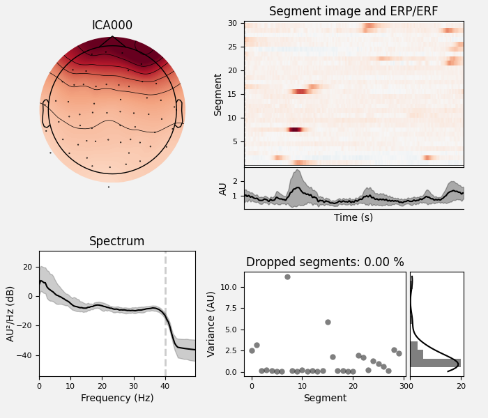
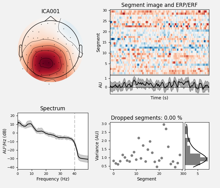
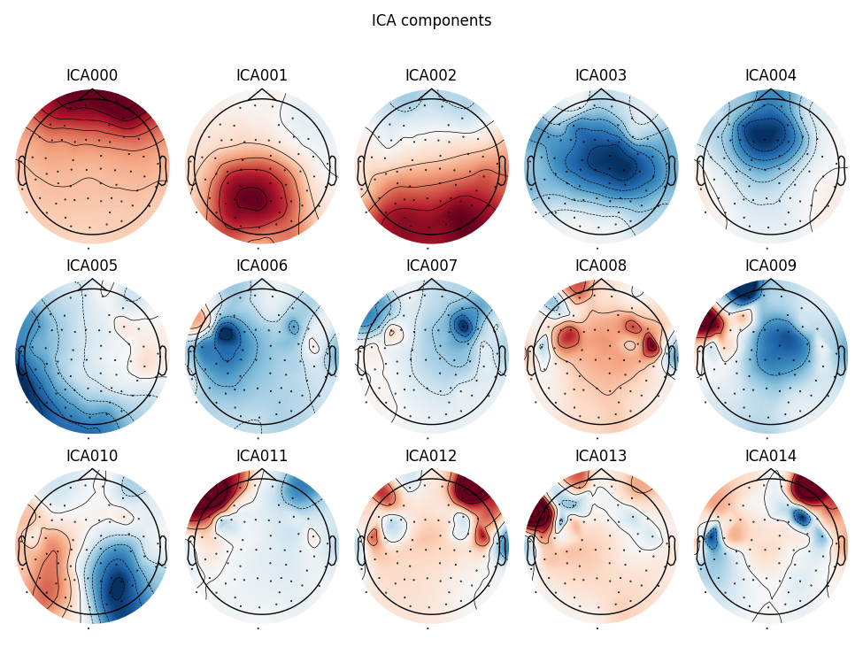
Here we can pretty clearly see that the first component (ICA000) captures the EOG signal quite well, and the second component (ICA001) looks a lot like a heartbeat (for more info on visually identifying Independent Components, this EEGLAB tutorial is a good resource). We can also visualize the scalp field distribution of each component using plot_components. These are interpolated based on the values in the ICA mixing matrix:

ica.plot_components()

# blinks
ica.plot_overlay(raw, exclude=[0], picks="eeg")

• 
• 

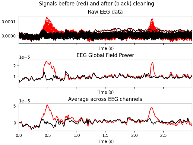
Applying ICA to Raw instance
    Transforming to ICA space (15 components)
    Zeroing out 1 ICA component
    Projecting back using 59 PCA components

We can also plot some diagnostics of each IC using plot_properties:

ica.plot_properties(raw, picks=[0, 1])

# Selecting ICA components automatically
# ~~~~~~~~~~~~~~~~~~~~~~~~~~~~~~~~~~~~~~
#
# Now that we've explored what components need to be removed, we can
# apply the automatic ICA component labeling algorithm, which will
# assign a probability value for each component being one of:
#
# - brain
# - muscle artifact
# - eye blink
# - heart beat
# - line noise
# - channel noise
# - other
#
# The output of the ICLabel ``label_components`` function produces
# predicted probability values for each of these classes in that order.
#
# To start this process, we will compute features of each ICA
# component to be fed into our classification model. This is
# done automatically underneath the hood. An autocorrelation,
# power spectral density and topographic map feature is fed
# into a 3-head neural network that has been pretrained.
# See :footcite:`iclabel2019` for full details.

ic_labels = label_components(raw, ica, method="iclabel")
print(ic_labels)

# We can extract the labels of each component and exclude
# non-brain classified components, keeping 'brain' and 'other'.
# "Other" is a catch-all that for non-classifiable components.
# We will ere on the side of caution and assume we cannot blindly remove these.
labels = ic_labels["labels"]
exclude_idx = [idx for idx, label in enumerate(labels) if label not in ["brain", "other"]]
print(f"Excluding these ICA components: {exclude_idx}")

• 
• 

    Using multitaper spectrum estimation with 7 DPSS windows
Not setting metadata
30 matching events found
No baseline correction applied
0 projection items activated
Not setting metadata
30 matching events found
No baseline correction applied
0 projection items activated
/home/scheltie/git/mne-tools/mne-icalabel/mne_icalabel/iclabel/features.py:46: RuntimeWarning: The provided Raw instance does not seems to be referenced to a common average reference (CAR). ICLabel was designed to classify features extracted from an EEG dataset referenced to a CAR (see the 'set_eeg_reference()' method for Raw and Epochs instances).
  warn(
/home/scheltie/git/mne-tools/mne-icalabel/mne_icalabel/iclabel/features.py:54: RuntimeWarning: The provided Raw instance is not filtered between 1 and 100 Hz. ICLabel was designed to classify features extracted from an EEG dataset bandpass filtered between 1 and 100 Hz (see the 'filter()' method for Raw and Epochs instances).
  warn(
/home/scheltie/git/mne-tools/mne-icalabel/mne_icalabel/iclabel/features.py:67: RuntimeWarning: The provided ICA instance was fitted with a 'fastica' algorithm. ICLabel was designed with extended infomax ICA decompositions. To use the extended infomax algorithm, use the 'mne.preprocessing.ICA' instance with the arguments 'ICA(method='infomax', fit_params=dict(extended=True))' (scikit-learn) or 'ICA(method='picard', fit_params=dict(ortho=False, extended=True))' (python-picard).
  warn(
NOTE: pick_channels() is a legacy function. New code should use inst.pick(...).
/home/scheltie/git/mne-tools/mne-icalabel/mne_icalabel/iclabel/utils.py:139: RuntimeWarning: divide by zero encountered in log
  g = np.square(d) * (np.log(d) - 1)  # % Green's function.
/home/scheltie/git/mne-tools/mne-icalabel/mne_icalabel/iclabel/utils.py:139: RuntimeWarning: invalid value encountered in multiply
  g = np.square(d) * (np.log(d) - 1)  # % Green's function.
{'y_pred_proba': array([0.87586254, 0.9996909 , 0.9081913 , 0.9517963 , 0.9620735 ,
       0.6919646 , 0.5977515 , 0.5735682 , 0.68124413, 0.7705698 ,
       0.99767613, 0.35102308, 0.5798828 , 0.6460217 , 0.75504196],
      dtype=float32), 'labels': ['eye blink', 'brain', 'brain', 'brain', 'brain', 'brain', 'other', 'other', 'other', 'other', 'brain', 'eye blink', 'muscle artifact', 'other', 'muscle artifact']}
Excluding these ICA components: [0, 11, 12, 14]

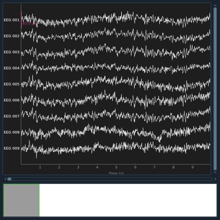
Now that the exclusions have been set, we can reconstruct the sensor signals with artifacts removed using the apply method (remember, we’re applying the ICA solution from the filtered data to the original unfiltered signal). Plotting the original raw data alongside the reconstructed data shows that the heartbeat and blink artifacts are repaired.

# ica.apply() changes the Raw object in-place, so let's make a copy first:
reconst_raw = raw.copy()
ica.apply(reconst_raw, exclude=exclude_idx)

raw.plot(order=artifact_picks, n_channels=len(artifact_picks), show_scrollbars=False)
reconst_raw.plot(order=artifact_picks, n_channels=len(artifact_picks), show_scrollbars=False)
del reconst_raw

• 
• 

Applying ICA to Raw instance
    Transforming to ICA space (15 components)
    Zeroing out 4 ICA components
    Projecting back using 59 PCA components

References

[1]

Luca Pion-Tonachini, Ken Kreutz-Delgado, and Scott Makeig. Iclabel: an automated electroencephalographic independent component classifier, dataset, and website. NeuroImage, 198:181–197, 2019. URL: https://www.sciencedirect.com/science/article/pii/S1053811919304185, doi:https://doi.org/10.1016/j.neuroimage.2019.05.026.

[2]

Irene Winkler, Stefan Debener, Klaus-Robert Müller, and Michael Tangermann. On the influence of high-pass filtering on ICA-based artifact reduction in EEG-ERP. In Proceedings of EMBC-2015, 4101–4105. Milan, 2015. IEEE. doi:10.1109/EMBC.2015.7319296.

Estimated memory usage: 283 MB