mne.Evoked#
- class mne.Evoked(fname, condition=None, proj=True, kind='average', allow_maxshield=False, *, verbose=None)[source]#
Evoked data.
- Parameters:
- fnamepath-like
Name of evoked/average FIF file to load. If None no data is loaded.
- condition
int, orstr Dataset ID number (int) or comment/name (str). Optional if there is only one data set in file.
- projbool, optional
Apply SSP projection vectors.
- kind
str Either
'average'or'standard_error'. The type of data to read. Only used if ‘condition’ is a str.- allow_maxshieldbool |
str(defaultFalse) If True, allow loading of data that has been recorded with internal active compensation (MaxShield). Data recorded with MaxShield should generally not be loaded directly, but should first be processed using SSS/tSSS to remove the compensation signals that may also affect brain activity. Can also be
"yes"to load without eliciting a warning.- verbosebool |
str|int|None Control verbosity of the logging output. If
None, use the default verbosity level. See the logging documentation andmne.verbose()for details. Should only be passed as a keyword argument.
- Attributes:
- info
mne.Info The
mne.Infoobject with information about the sensors and methods of measurement.ch_nameslistofstrChannel names.
- nave
int Number of averaged epochs.
kindstrThe data kind.
- comment
str Comment on dataset. Can be the condition.
dataarrayof shape (n_channels, n_times)The data matrix.
- first
int First time sample.
- last
int Last time sample.
tminfloatFirst time point.
tmaxfloatLast time point.
timesarrayTime vector in seconds.
- baseline
None|tupleof length 2 This attribute reflects whether the data has been baseline-corrected (it will be a
tuplethen) or not (it will beNone).
- info
Methods
__contains__(ch_type)Check channel type membership.
__neg__()Negate channel responses.
add_channels(add_list[, force_update_info])Append new channels from other MNE objects to the instance.
add_proj(projs[, remove_existing, verbose])Add SSP projection vectors.
add_reference_channels(ref_channels)Add reference channels to data that consists of all zeros.
animate_topomap(*[, times, average, ...])Make animation of evoked data as topomap timeseries.
anonymize([daysback, keep_his, verbose])Anonymize measurement information in place.
apply_baseline([baseline, verbose])Baseline correct evoked data.
apply_function(fun[, picks, dtype, n_jobs, ...])Apply a function to a subset of channels.
apply_hilbert([picks, envelope, n_jobs, ...])Compute analytic signal or envelope for a subset of channels/vertices.
apply_proj([verbose])Apply the signal space projection (SSP) operators to the data.
as_type([ch_type, mode])Compute virtual evoked using interpolated fields.
compute_psd([method, fmin, fmax, tmin, ...])Perform spectral analysis on sensor data.
compute_tfr(method, freqs, *[, tmin, tmax, ...])Compute a time-frequency representation of evoked data.
copy()Copy the instance of evoked.
crop([tmin, tmax, include_tmax, verbose])Crop data to a given time interval.
decimate(decim[, offset, verbose])Decimate the time-series data.
del_proj([idx])Remove SSP projection vector.
detrend([order, picks])Detrend data.
drop_channels(ch_names[, on_missing])Drop channel(s).
export(fname[, fmt, overwrite, verbose])Export Evoked to external formats.
filter(l_freq, h_freq[, picks, ...])Filter a subset of channels/vertices.
get_channel_types([picks, unique, only_data_chs])Get a list of channel type for each channel.
get_data([picks, units, tmin, tmax])Get evoked data as 2D array.
Get a DigMontage from instance.
get_peak([ch_type, tmin, tmax, mode, ...])Get location and latency of peak amplitude.
interpolate_bads([reset_bads, mode, origin, ...])Interpolate bad MEG and EEG channels.
interpolate_to(sensors[, origin, method, ...])Interpolate data onto a new sensor configuration.
pick(picks[, exclude, verbose])Pick a subset of channels.
pick_channels(ch_names[, ordered, verbose])pick_types([meg, eeg, stim, eog, ecg, emg, ...])plot([picks, exclude, unit, show, ylim, ...])Plot evoked data using butterfly plots.
plot_field(surf_maps[, time, time_label, ...])Plot MEG/EEG fields on head surface and helmet in 3D.
plot_image([picks, exclude, unit, show, ...])Plot evoked data as images.
plot_joint([times, title, picks, exclude, ...])Plot evoked data as butterfly plot and add topomaps for time points.
plot_projs_topomap([ch_type, sensors, ...])Plot SSP vector.
plot_psd([fmin, fmax, tmin, tmax, picks, ...])Plot power or amplitude spectra.
plot_psd_topo([tmin, tmax, fmin, fmax, ...])plot_psd_topomap([bands, tmin, tmax, ...])plot_sensors([kind, ch_type, title, ...])Plot sensor positions.
plot_topo([layout, layout_scale, color, ...])Plot 2D topography of evoked responses.
plot_topomap([times, average, ch_type, ...])Plot topographic maps of specific time points of evoked data.
plot_white(noise_cov[, show, rank, ...])Plot whitened evoked response.
rename_channels(mapping[, allow_duplicates, ...])Rename channels.
reorder_channels(ch_names)Reorder channels.
resample(sfreq, *[, npad, window, n_jobs, ...])Resample data.
save(fname, *[, overwrite, verbose])Save evoked data to a file.
savgol_filter(h_freq[, verbose])Filter the data using Savitzky-Golay polynomial method.
set_channel_types(mapping, *[, ...])Specify the sensor types of channels.
set_eeg_reference([ref_channels, ...])Specify which reference to use for EEG data.
set_meas_date(meas_date)Set the measurement start date.
set_montage(montage[, match_case, ...])Set EEG/sEEG/ECoG/DBS/fNIRS channel positions and digitization points.
shift_time(tshift[, relative])Shift time scale in epoched or evoked data.
time_as_index(times[, use_rounding])Convert time to indices.
to_data_frame([picks, index, scalings, ...])Export data in tabular structure as a pandas DataFrame.
Notes
Evoked objects can only contain the average of a single set of conditions.
- __contains__(ch_type)[source]#
Check channel type membership.
- Parameters:
- ch_type
str Channel type to check for. Can be e.g.
'meg','eeg','stim', etc.
- ch_type
- Returns:
- inbool
Whether or not the instance contains the given channel type.
Examples
Channel type membership can be tested as:
>>> 'meg' in inst
True
>>> 'seeg' in inst
False
- __neg__()[source]#
Negate channel responses.
- Returns:
- evoked_neginstance of
Evoked The Evoked instance with channel data negated and ‘-’ prepended to the comment.
- evoked_neginstance of
- add_channels(add_list, force_update_info=False)[source]#
Append new channels from other MNE objects to the instance.
- Parameters:
- add_list
list A list of MNE objects to append to the current instance. The channels contained in the other instances are appended to the channels of the current instance. Therefore, all other instances must be of the same type as the current object. See notes on how to add data coming from an array.
- force_update_infobool
If True, force the info for objects to be appended to match the values of the current instance. This should generally only be used when adding stim channels for which important metadata won’t be overwritten.
New in v0.12.
- add_list
- Returns:
- instsame
typeas the input data The modified instance.
- instsame
See also
Notes
If
selfis a Raw instance that has been preloaded into anumpy.memmapinstance, the memmap will be resized.This function expects an MNE object to be appended (e.g.
Raw,Epochs,Evoked). If you simply want to add a channel based on values of an np.ndarray, you need to create aRawArray. See <https://mne.tools/mne-project-template/auto_examples/plot_mne_objects_from_arrays.html>`_
- add_proj(projs, remove_existing=False, verbose=None)[source]#
Add SSP projection vectors.
- Parameters:
- projs
list List with projection vectors.
- remove_existingbool
Remove the projection vectors currently in the file.
- verbosebool |
str|int|None Control verbosity of the logging output. If
None, use the default verbosity level. See the logging documentation andmne.verbose()for details. Should only be passed as a keyword argument.
- projs
- Returns:
- selfsame
typeas the input data The data container.
- selfsame
Examples using
add_proj:
- add_reference_channels(ref_channels)[source]#
Add reference channels to data that consists of all zeros.
Adds reference channels to data that were not included during recording. This is useful when you need to re-reference your data to different channels. These added channels will consist of all zeros.
- animate_topomap(*, times=None, average=None, ch_type=None, scalings=None, proj=False, sensors=True, show_names=False, mask=None, mask_params=None, contours=6, outlines='head', sphere=None, image_interp='cubic', extrapolate='auto', border='mean', res=64, size=1.0, cmap=None, vlim=(None, None), cnorm=None, colorbar=True, cbar_fmt='%3.1f', units=None, axes=None, time_unit='s', time_format=None, frame_rate=None, butterfly=False, blit=True, show=True, vmin=None, vmax=None, verbose=None)[source]#
Make animation of evoked data as topomap timeseries.
The animation can be paused/resumed with left mouse button. Left and right arrow keys can be used to move backward or forward in time.
- Parameters:
- times
arrayoffloat|None The time points to plot. If None (default), 10 evenly spaced samples are calculated over the evoked time series.
- average
float| array_like offloat, shape (n_times,) |None The time window (in seconds) around a given time point to be used for averaging. For example, 0.2 would translate into a time window that starts 0.1 s before and ends 0.1 s after the given time point. If the time window exceeds the duration of the data, it will be clipped. Different time windows (one per time point) can be provided by passing an
array-likeobject (e.g.,[0.1, 0.2, 0.3]). IfNone(default), no averaging will take place.Changed in version 1.1: Support for
array-likeinput.- ch_type‘mag’ | ‘grad’ | ‘planar1’ | ‘planar2’ | ‘eeg’ |
None The channel type to plot. For
'grad', the gradiometers are collected in pairs and the RMS for each pair is plotted. IfNonethe first available channel type from order shown above is used. Defaults toNone.- scalings
dict|float|None The scalings of the channel types to be applied for plotting. If None, defaults to
dict(eeg=1e6, grad=1e13, mag=1e15).- projbool | ‘interactive’ | ‘reconstruct’
If true SSP projections are applied before display. If
'interactive', a check box for reversible selection of SSP projection vectors will be shown. If'reconstruct', projection vectors will be applied and then M/EEG data will be reconstructed via field mapping to reduce the signal bias caused by projection.Changed in version 0.21: Support for ‘reconstruct’ was added.
- sensorsbool |
str Whether to add markers for sensor locations. If
str, should be a valid matplotlib format string (e.g.,'r+'for red plusses, see the Notes section ofplot()). IfTrue(the default), black circles will be used.- show_namesbool |
callable() If
True, show channel names next to each sensor marker. If callable, channel names will be formatted using the callable; e.g., to delete the prefix ‘MEG ‘ from all channel names, pass the functionlambda x: x.replace('MEG ', ''). Ifmaskis notNone, only non-masked sensor names will be shown.- mask
ndarrayof bool, shape (n_channels, n_times) |None Array indicating channel-time combinations to highlight with a distinct plotting style (useful for, e.g. marking which channels at which times a statistical test of the data reaches significance). Array elements set to
Truewill be plotted with the parameters given inmask_params. Defaults toNone, equivalent to an array of allFalseelements.- mask_params
dict|None Additional plotting parameters for plotting significant sensors. Default (None) equals:
dict(marker='o', markerfacecolor='w', markeredgecolor='k',
        linewidth=0, markersize=4)
- contours
int| array_like The number of contour lines to draw. If
0, no contours will be drawn. If a positive integer, that number of contour levels are chosen using the matplotlib tick locator (may sometimes be inaccurate, use array for accuracy). If array-like, the array values are used as the contour levels. The values should be in µV for EEG, fT for magnetometers and fT/m for gradiometers. Ifcolorbar=True, the colorbar will have ticks corresponding to the contour levels. Default is6.- outlines‘head’ |
dict|None The outlines to be drawn. If ‘head’, the default head scheme will be drawn. If dict, each key refers to a tuple of x and y positions, the values in ‘mask_pos’ will serve as image mask. Alternatively, a matplotlib patch object can be passed for advanced masking options, either directly or as a function that returns patches (required for multi-axis plots). If None, nothing will be drawn. Defaults to ‘head’.
- sphere
float| array_like offloat| instance ofConductorModel|str|listofstr|None The sphere parameters to use for the head outline. Can be array-like of shape (4,) to give the X/Y/Z origin and radius in meters, or a single float to give just the radius (origin assumed 0, 0, 0). Can also be an instance of a spherical
ConductorModelto use the origin and radius from that object. Can also be astr, in which case:'auto': the sphere is fit to external digitization points first, and to external + EEG digitization points if the former fails.'eeglab': the head circle is defined by EEG electrodes'Fpz','Oz','T7', and'T8'(if'Fpz'is not present, it will be approximated from the coordinates of'Oz').'extra': the sphere is fit to external digitization points.'eeg': the sphere is fit to EEG digitization points.'cardinal': the sphere is fit to cardinal digitization points.'hpi': the sphere is fit to HPI coil digitization points.
Can also be a list of
str, in which case the sphere is fit to the specified digitization points, which can be any combination of'extra','eeg','cardinal', and'hpi', as specified above.None(the default) is equivalent to'auto'when enough extra digitization points are available, and (0, 0, 0, 0.095) otherwise.New in v0.20.
Changed in version 1.1: Added
'eeglab'option.Changed in version 1.11: Added
'extra','eeg','cardinal','hpi'and list ofstroptions.- image_interp
str The image interpolation to be used. Options are
'cubic'(default) to usescipy.interpolate.CloughTocher2DInterpolator,'nearest'to usescipy.spatial.Voronoior'linear'to usescipy.interpolate.LinearNDInterpolator.- extrapolate
str Options:
'box'Extrapolate to four points placed to form a square encompassing all data points, where each side of the square is three times the range of the data in the respective dimension.
'local'(default for MEG sensors)Extrapolate only to nearby points (approximately to points closer than median inter-electrode distance). This will also set the mask to be polygonal based on the convex hull of the sensors.
'head'(default for non-MEG sensors)Extrapolate out to the edges of the clipping circle. This will be on the head circle when the sensors are contained within the head circle, but it can extend beyond the head when sensors are plotted outside the head circle.
- border
float| ‘mean’ Value to extrapolate to on the topomap borders. If
'mean'(default), then each extrapolated point has the average value of its neighbours.- res
int The resolution of the topomap image (number of pixels along each side).
- size
float Side length of each subplot in inches.
- cmapmatplotlib colormap | (colormap, bool) | ‘interactive’ |
None Colormap to use. If
tuple, the first value indicates the colormap to use and the second value is a boolean defining interactivity. In interactive mode the colors are adjustable by clicking and dragging the colorbar with left and right mouse button. Left mouse button moves the scale up and down and right mouse button adjusts the range. Hitting space bar resets the range. Up and down arrows can be used to change the colormap. IfNone,'Reds'is used for data that is either all-positive or all-negative, and'RdBu_r'is used otherwise.'interactive'is equivalent to(None, True). Defaults toNone.Warning
Interactive mode works smoothly only for a small amount of topomaps. Interactive mode is disabled by default for more than 2 topomaps.
- vlim
tupleof length 2 | “joint” Lower and upper bounds of the colormap, typically a numeric value in the same units as the data. Elements of the
tuplemay also be callable functions which take in aNumPy arrayand return a scalar.If both entries are
None, the bounds are set at ± the maximum absolute value of the data (yielding a colormap with midpoint at 0), or(0, max(abs(data)))if the (possibly baselined) data are all-positive. ProvidingNonefor just one entry will set the corresponding boundary at the min/max of the data. Ifvlim="joint", will compute the colormap limits jointly across all topomaps of the same channel type (instead of separately for each topomap), using the min/max of the data for that channel type. Defaults to(None, None).- cnorm
matplotlib.colors.Normalize|None How to normalize the colormap. If
None, standard linear normalization is performed. If notNone,vminandvmaxwill be ignored. See Matplotlib docs for more details on colormap normalization, and the ERDs example for an example of its use.- colorbarbool
Plot a colorbar in the rightmost column of the figure.
- cbar_fmt
str Formatting string for colorbar tick labels. See Format specification mini-language for details.
- units
dict|str|None The units to use for the colorbar label. Ignored if
colorbar=False. IfNoneandscalings=Nonethe unit is automatically determined, otherwise the label will be “AU” indicating arbitrary units. Default isNone.- axes
listofmatplotlib.axes.Axes|None The axes to use for plotting. Must have one axis for the topomap, then one for the colorbar (if
colorbar=True), then one for the butterfly axes (ifbutterfly=True).- time_unit
str The units for the time axis, can be “ms” or “s” (default).
- time_format
str|None String format for topomap values. Defaults (None) to “%01d ms” if
time_unit='ms', “%0.3f s” iftime_unit='s', and “%g” otherwise. Can be an empty string to omit the time label.- frame_rate
int|None Frame rate for the animation in Hz. If None, frame rate = sfreq / 10. Defaults to None.
- butterflybool
Whether to plot the data as butterfly plot under the topomap. Defaults to False.
- blitbool
Whether to use blit to optimize drawing. In general, it is recommended to use blit in combination with
show=True. If you intend to save the animation it is better to disable blit. Defaults to True.- showbool
Whether to show the animation. Defaults to True.
- vmin
float|None Deprecated, use
vlim=(vmin, vmax)instead.- vmax
float|None Deprecated, use
vlim=(vmin, vmax)instead.- verbosebool |
str|int|None Control verbosity of the logging output. If
None, use the default verbosity level. See the logging documentation andmne.verbose()for details. Should only be passed as a keyword argument.
- times
- Returns:
- figinstance of
matplotlib.figure.Figure The figure.
- animinstance of
matplotlib.animation.FuncAnimation Animation of the topomap.
- figinstance of
Notes
Changed in version 1.13.0: The
vminandvmaxparameters were deprecated in favor of a singlevlimparameter, and parameters were added and reordered to followplot_topomap().New in v0.12.0.
Examples using
animate_topomap:
- anonymize(daysback=None, keep_his=False, verbose=None)[source]#
Anonymize measurement information in place.
- Parameters:
- daysback
int|None Number of days to subtract from all dates. If
None(default), the acquisition date,info['meas_date'], will be set toJanuary 1ˢᵗ, 2000. This parameter is ignored ifinfo['meas_date']isNone(i.e., no acquisition date has been set).- keep_hisbool | “his_id” | “sex” | “hand” | sequence of {“his_id”, “sex”, “hand”}
If
True,his_id,sex, andhandofsubject_infowill not be overwritten. IfFalse, these fields will be anonymized. If"his_id","sex", or"hand"(or any combination thereof in a sequence), only those fields will not be anonymized. Defaults toFalse.Warning
Setting
keep_histo anything other thanFalsemay result ininfonot being fully anonymized. Use with caution.Changed in version 1.12: Added support for sequence of
str.- verbosebool |
str|int|None Control verbosity of the logging output. If
None, use the default verbosity level. See the logging documentation andmne.verbose()for details. Should only be passed as a keyword argument.
- daysback
- Returns:
- instsame
typeas the input data The modified instance.
- instsame
Notes
Removes potentially identifying information if it exists in
info. Specifically for each of the following we use:- meas_date, file_id, meas_id
A default value, or as specified by
daysback.
- subject_info
Default values, except for ‘birthday’, which is adjusted to maintain the subject age. If
keep_hisis notFalse, then the fields ‘his_id’, ‘sex’, and ‘hand’ are not anonymized, depending on the value ofkeep_his.
- experimenter, proj_name, description
Default strings.
- utc_offset
None.
- proj_id
Zeros.
- proc_history
Dates use the
meas_datelogic, and experimenter a default string.
- helium_info, device_info
Dates use the
meas_datelogic, meta info uses defaults.
If
info['meas_date']isNone, it will remainNoneduring processing the above fields.Operates in place.
New in v0.13.0.
- apply_baseline(baseline=(None, 0), *, verbose=None)[source]#
Baseline correct evoked data.
- Parameters:
- baseline
None|tupleof length 2 The time interval to consider as “baseline” when applying baseline correction. If
None, do not apply baseline correction. If a tuple(a, b), the interval is betweenaandb(in seconds), including the endpoints. IfaisNone, the beginning of the data is used; and ifbisNone, it is set to the end of the data. If(None, None), the entire time interval is used.Note
The baseline
(a, b)includes both endpoints, i.e. all timepointstsuch thata <= t <= b.Correction is applied to each channel individually in the following way:
Calculate the mean signal of the baseline period.
Subtract this mean from the entire
Evoked.
Defaults to
(None, 0), i.e. beginning of the data until time point zero.- verbosebool |
str|int|None Control verbosity of the logging output. If
None, use the default verbosity level. See the logging documentation andmne.verbose()for details. Should only be passed as a keyword argument.
- baseline
- Returns:
- evokedinstance of
Evoked The baseline-corrected Evoked object.
- evokedinstance of
Notes
Baseline correction can be done multiple times.
New in v0.13.0.
Examples using
apply_baseline:
- apply_function(fun, picks=None, dtype=None, n_jobs=None, channel_wise=True, *, verbose=None, **kwargs)[source]#
Apply a function to a subset of channels.
The function
funis applied to the channels defined inpicks. The evoked object’s data is modified in-place. If the function returns a different data type (e.g.numpy.complex128) it must be specified using thedtypeparameter, which causes the data type of all the data to change (even if the function is only applied to channels inpicks).Note
If
n_jobs> 1, more memory is required aslen(picks) * n_timesadditional time points need to be temporarily stored in memory.Note
If the data type changes (
dtype != None), more memory is required since the original and the converted data needs to be stored in memory.- Parameters:
- fun
callable() A function to be applied to the channels. The first argument of fun has to be a timeseries (
numpy.ndarray). The function must operate on an array of shape(n_times,)because it will apply channel-wise. The function must return anndarrayshaped like its input.Note
If
channel_wise=True, one can optionally access the index and/or the name of the currently processed channel within the applied function. This can enable tailored computations for different channels. To use this feature, addch_idxand/orch_nameas additional argument(s) to your function definition.- picks
str| array_like |slice|None Channels to include. Slices and lists of integers will be interpreted as channel indices. In lists, channel type strings (e.g.,
['meg',
'eeg']
) will pick channels of those types, channel name strings (e.g.,['MEG0111', 'MEG2623']will pick the given channels. Can also be the string values'all'to pick all channels, or'data'to pick data channels. None (default) will pick all data channels (excluding reference MEG channels). Note that channels ininfo['bads']will be included if their names or indices are explicitly provided.- dtype
numpy.dtype Data type to use after applying the function. If None (default) the data type is not modified.
- n_jobs
int|None The number of jobs to run in parallel. If
-1, it is set to the number of CPU cores. Requires thejoblibpackage.None(default) is a marker for ‘unset’ that will be interpreted asn_jobs=1(sequential execution) unless the call is performed under ajoblib.parallel_configcontext manager that sets another value forn_jobs. Ignored ifchannel_wise=Falseas the workload is split across channels.- channel_wisebool
Whether to apply the function to each channel individually. If
False, the function will be applied to all channels at once. DefaultTrue.New in v1.6.
- verbosebool |
str|int|None Control verbosity of the logging output. If
None, use the default verbosity level. See the logging documentation andmne.verbose()for details. Should only be passed as a keyword argument.- **kwargs
dict Additional keyword arguments to pass to
fun.
- fun
- Returns:
- selfinstance of
Evoked The evoked object with transformed data.
- selfinstance of
- apply_hilbert(picks=None, envelope=False, n_jobs=None, n_fft='auto', *, verbose=None)[source]#
Compute analytic signal or envelope for a subset of channels/vertices.
- Parameters:
- picks
str| array_like |slice|None Channels to include. Slices and lists of integers will be interpreted as channel indices. In lists, channel type strings (e.g.,
['meg',
'eeg']
) will pick channels of those types, channel name strings (e.g.,['MEG0111', 'MEG2623']will pick the given channels. Can also be the string values'all'to pick all channels, or'data'to pick data channels. None (default) will pick all data channels (excluding reference MEG channels). Note that channels ininfo['bads']will be included if their names or indices are explicitly provided.- envelopebool
Compute the envelope signal of each channel/vertex. Default False. See Notes.
- n_jobs
int|None The number of jobs to run in parallel. If
-1, it is set to the number of CPU cores. Requires thejoblibpackage.None(default) is a marker for ‘unset’ that will be interpreted asn_jobs=1(sequential execution) unless the call is performed under ajoblib.parallel_configcontext manager that sets another value forn_jobs.- n_fft
int|None|str Points to use in the FFT for Hilbert transformation. The signal will be padded with zeros before computing Hilbert, then cut back to original length. If None, n == self.n_times. If ‘auto’, the next highest fast FFT length will be use.
- verbosebool |
str|int|None Control verbosity of the logging output. If
None, use the default verbosity level. See the logging documentation andmne.verbose()for details. Should only be passed as a keyword argument.
- picks
- Returns:
- selfinstance of
Raw,Epochs,EvokedorSourceEstimate The raw object with transformed data.
- selfinstance of
Notes
Parameters
If
envelope=False, the analytic signal for the channels/vertices defined inpicksis computed and the data of the Raw object is converted to a complex representation (the analytic signal is complex valued).If
envelope=True, the absolute value of the analytic signal for the channels/vertices defined inpicksis computed, resulting in the envelope signal.If envelope=False, more memory is required since the original raw data as well as the analytic signal have temporarily to be stored in memory. If n_jobs > 1, more memory is required as
len(picks) * n_timesadditional time points need to be temporarily stored in memory.Also note that the
n_fftparameter will allow you to pad the signal with zeros before performing the Hilbert transform. This padding is cut off, but it may result in a slightly different result (particularly around the edges). Use at your own risk.Analytic signal
The analytic signal “x_a(t)” of “x(t)” is:
x_a = F^{-1}(F(x) 2U) = x + i y
where “F” is the Fourier transform, “U” the unit step function, and “y” the Hilbert transform of “x”. One usage of the analytic signal is the computation of the envelope signal, which is given by “e(t) = abs(x_a(t))”. Due to the linearity of Hilbert transform and the MNE inverse solution, the enevlope in source space can be obtained by computing the analytic signal in sensor space, applying the MNE inverse, and computing the envelope in source space.
- apply_proj(verbose=None)[source]#
Apply the signal space projection (SSP) operators to the data.
- Parameters:
- verbosebool |
str|int|None Control verbosity of the logging output. If
None, use the default verbosity level. See the logging documentation andmne.verbose()for details. Should only be passed as a keyword argument.
- verbosebool |
- Returns:
- selfsame
typeas the input data The instance.
- selfsame
Notes
Once the projectors have been applied, they can no longer be removed. It is usually not recommended to apply the projectors at too early stages, as they are applied automatically later on (e.g. when computing inverse solutions). Hint: using the copy method individual projection vectors can be tested without affecting the original data. With evoked data, consider the following example:
projs_a = mne.read_proj('proj_a.fif')
projs_b = mne.read_proj('proj_b.fif')
# add the first, copy, apply and see ...
evoked.add_proj(a).copy().apply_proj().plot()
# add the second, copy, apply and see ...
evoked.add_proj(b).copy().apply_proj().plot()
# drop the first and see again
evoked.copy().del_proj(0).apply_proj().plot()
evoked.apply_proj()  # finally keep both
Examples using
apply_proj:
- as_type(ch_type='grad', mode='fast')[source]#
Compute virtual evoked using interpolated fields.
Warning
Using virtual evoked to compute inverse can yield unexpected results. The virtual channels have
'_v'appended at the end of the names to emphasize that the data contained in them are interpolated.- Parameters:
- Returns:
- evokedinstance of
mne.Evoked The transformed evoked object containing only virtual channels.
- evokedinstance of
Notes
This method returns a copy and does not modify the data it operates on. It also returns an EvokedArray instance.
New in v0.9.0.
Examples using
as_type:
- property ch_names#
Channel names.
- property compensation_grade#
The current gradient compensation grade.
- compute_psd(method='multitaper', fmin=0, fmax=inf, tmin=None, tmax=None, picks=None, proj=False, remove_dc=True, exclude=(), *, n_jobs=1, verbose=None, **method_kw)[source]#
Perform spectral analysis on sensor data.
- Parameters:
- method
'welch'|'multitaper' Spectral estimation method.
'welch'uses Welch’s method [1],'multitaper'uses DPSS tapers [2]. Default is'multitaper'.- fmin, fmax
float The lower- and upper-bound on frequencies of interest. Default is
fmin=0, fmax=np.inf(spans all frequencies present in the data).- tmin, tmax
float|None First and last times to include, in seconds.
Noneuses the first or last time present in the data. Default istmin=None, tmax=None(all times).- picks
str| array_like |slice|None Channels to include. Slices and lists of integers will be interpreted as channel indices. In lists, channel type strings (e.g.,
['meg',
'eeg']
) will pick channels of those types, channel name strings (e.g.,['MEG0111', 'MEG2623']will pick the given channels. Can also be the string values'all'to pick all channels, or'data'to pick data channels. None (default) will pick good data channels (excluding reference MEG channels). Note that channels ininfo['bads']will be included if their names or indices are explicitly provided.- projbool
Whether to apply SSP projection vectors before spectral estimation. Default is
False.- remove_dcbool
If
True, the mean is subtracted from each segment before computing its spectrum.- exclude
listofstr| ‘bads’ Channel names to exclude. If
'bads', channels ininfo['bads']are excluded; pass an empty list to include all channels (including “bad” channels, if any).- n_jobs
int|None The number of jobs to run in parallel. If
-1, it is set to the number of CPU cores. Requires thejoblibpackage.None(default) is a marker for ‘unset’ that will be interpreted asn_jobs=1(sequential execution) unless the call is performed under ajoblib.parallel_configcontext manager that sets another value forn_jobs.- verbosebool |
str|int|None Control verbosity of the logging output. If
None, use the default verbosity level. See the logging documentation andmne.verbose()for details. Should only be passed as a keyword argument.- **method_kw
Additional keyword arguments passed to the spectral estimation function (e.g.,
n_fft, n_overlap, n_per_seg, average, windowfor Welch method, orbandwidth, adaptive, low_bias, normalizationfor multitaper method). Seepsd_array_welch()andpsd_array_multitaper()for details. Note that for Welch method ifn_fftis unspecified its default will be the smaller of2048or the number of available time samples (taking into accounttminandtmax), not256as inpsd_array_welch().
- method
- Returns:
- spectruminstance of
Spectrum The spectral representation of the data.
- spectruminstance of
Notes
New in v1.2.
References
Examples using
compute_psd:
The Spectrum and EpochsSpectrum classes: frequency-domain data
The Spectrum and EpochsSpectrum classes: frequency-domain data
- compute_tfr(method, freqs, *, tmin=None, tmax=None, picks=None, proj=False, output='power', decim=1, n_jobs=None, verbose=None, **method_kw)[source]#
Compute a time-frequency representation of evoked data.
- Parameters:
- method
'morlet'|'multitaper'|None Spectrotemporal power estimation method.
'morlet'uses Morlet wavelets,'multitaper'uses DPSS tapers [2].None(the default) only works when using__setstate__and will raise an error otherwise.- freqsarray_like |
None The frequencies at which to compute the power estimates. Must be an array of shape (n_freqs,).
None(the default) only works when using__setstate__and will raise an error otherwise.- tmin, tmax
float|None First and last times to include, in seconds.
Noneuses the first or last time present in the data. Default istmin=None, tmax=None(all times).- picks
str| array_like |slice|None Channels to include. Slices and lists of integers will be interpreted as channel indices. In lists, channel type strings (e.g.,
['meg',
'eeg']
) will pick channels of those types, channel name strings (e.g.,['MEG0111', 'MEG2623']will pick the given channels. Can also be the string values'all'to pick all channels, or'data'to pick data channels. None (default) will pick good data channels (excluding reference MEG channels). Note that channels ininfo['bads']will be included if their names or indices are explicitly provided.- projbool
Whether to apply SSP projection vectors before spectral estimation. Default is
False.- output
str What kind of estimate to return. Allowed values are
"complex","phase", and"power". Default is"power".- decim
int|slice Decimation factor, applied after time-frequency decomposition.
if
int, returnstfr[..., ::decim](keep only every Nth sample along the time axis).if
slice, returnstfr[..., decim](keep only the specified slice along the time axis).
Note
Decimation is done after convolutions and may create aliasing artifacts.
- n_jobs
int|None The number of jobs to run in parallel. If
-1, it is set to the number of CPU cores. Requires thejoblibpackage.None(default) is a marker for ‘unset’ that will be interpreted asn_jobs=1(sequential execution) unless the call is performed under ajoblib.parallel_configcontext manager that sets another value forn_jobs.- verbosebool |
str|int|None Control verbosity of the logging output. If
None, use the default verbosity level. See the logging documentation andmne.verbose()for details. Should only be passed as a keyword argument.- **method_kw
Additional keyword arguments passed to the spectrotemporal estimation function (e.g.,
n_cycles, use_fft, zero_meanfor Morlet method orn_cycles, use_fft, zero_mean, time_bandwidthfor multitaper method). Seetfr_array_morlet()andtfr_array_multitaper()for additional details.
- method
- Returns:
- tfrinstance of
AverageTFR The time-frequency-resolved power estimates of the data.
- tfrinstance of
Notes
New in v1.7.
References
- copy() Self[source]#
Copy the instance of evoked.
- Returns:
- evokedinstance of
Evoked A copy of the object.
- evokedinstance of
Examples using
copy:
Computing source timecourses with an XFit-like multi-dipole model
Computing source timecourses with an XFit-like multi-dipole model
Compute iterative reweighted TF-MxNE with multiscale time-frequency dictionary
Compute iterative reweighted TF-MxNE with multiscale time-frequency dictionary
Compute source power spectral density (PSD) of VectorView and OPM data
Compute source power spectral density (PSD) of VectorView and OPM data
Source localization with equivalent current dipole (ECD) fit
Source localization with equivalent current dipole (ECD) fit
Preprocessing optically pumped magnetometer (OPM) MEG data
Preprocessing optically pumped magnetometer (OPM) MEG data
- crop(tmin=None, tmax=None, include_tmax=True, verbose=None) Self[source]#
Crop data to a given time interval.
- Parameters:
- tmin
float|None Start time of selection in seconds.
- tmax
float|None End time of selection in seconds.
- include_tmaxbool
If True (default), include tmax. If False, exclude tmax (similar to how Python indexing typically works).
New in v0.19.
- verbosebool |
str|int|None Control verbosity of the logging output. If
None, use the default verbosity level. See the logging documentation andmne.verbose()for details. Should only be passed as a keyword argument.
- tmin
- Returns:
- instsame
typeas the input data The cropped time-series object, modified in-place.
- instsame
Notes
Unlike Python slices, MNE time intervals by default include both their end points;
crop(tmin, tmax)returns the intervaltmin <= t <= tmax. Passinclude_tmax=Falseto specify the half-open intervaltmin <= t < tmaxinstead.Examples using
crop:
Compute a sparse inverse solution using the Gamma-MAP empirical Bayesian method
Compute a sparse inverse solution using the Gamma-MAP empirical Bayesian method
Compute sparse inverse solution with mixed norm: MxNE and irMxNE
Compute sparse inverse solution with mixed norm: MxNE and irMxNE
Compute iterative reweighted TF-MxNE with multiscale time-frequency dictionary
Compute iterative reweighted TF-MxNE with multiscale time-frequency dictionary
Source localization with equivalent current dipole (ECD) fit
Source localization with equivalent current dipole (ECD) fit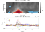
Non-parametric 1 sample cluster statistic on single trial power
Non-parametric 1 sample cluster statistic on single trial power
- property data#
The data matrix.
- decimate(decim, offset=0, *, verbose=None) Self[source]#
Decimate the time-series data.
- Parameters:
- decim
int Factor by which to subsample the data.
Warning
Low-pass filtering is not performed, this simply selects every Nth sample (where N is the value passed to
decim), i.e., it compresses the signal (see Notes). If the data are not properly filtered, aliasing artifacts may occur. See Resampling and decimating data for more information.- offset
int Apply an offset to where the decimation starts relative to the sample corresponding to t=0. The offset is in samples at the current sampling rate.
New in v0.12.
- verbosebool |
str|int|None Control verbosity of the logging output. If
None, use the default verbosity level. See the logging documentation andmne.verbose()for details. Should only be passed as a keyword argument.
- decim
- Returns:
- instMNE-object
The decimated object.
See also
Notes
For historical reasons,
decim/ “decimation” refers to simply subselecting samples from a given signal. This contrasts with the broader signal processing literature, where decimation is defined as (quoting [3], p. 172; which cites [4]):“… a general system for downsampling by a factor of M is the one shown in Figure 4.23. Such a system is called a decimator, and downsampling by lowpass filtering followed by compression [i.e, subselecting samples] has been termed decimation (Crochiere and Rabiner, 1983).”
Hence “decimation” in MNE is what is considered “compression” in the signal processing community.
Decimation can be done multiple times. For example,
inst.decimate(2).decimate(2)will be the same asinst.decimate(4).If
decimis 1, this method does not copy the underlying data.New in v0.10.0.
References
Examples using
decimate:
- del_proj(idx='all')[source]#
Remove SSP projection vector.
Note
The projection vector can only be removed if it is inactive (has not been applied to the data).
- Parameters:
- Returns:
- selfsame
typeas the input data The instance.
- selfsame
Examples using
del_proj:
- detrend(order=1, picks=None)[source]#
Detrend data.
This function operates in-place.
- Parameters:
- order
int Either 0 or 1, the order of the detrending. 0 is a constant (DC) detrend, 1 is a linear detrend.
- picks
str| array_like |slice|None Channels to include. Slices and lists of integers will be interpreted as channel indices. In lists, channel type strings (e.g.,
['meg',
'eeg']
) will pick channels of those types, channel name strings (e.g.,['MEG0111', 'MEG2623']will pick the given channels. Can also be the string values'all'to pick all channels, or'data'to pick data channels. None (default) will pick good data channels. Note that channels ininfo['bads']will be included if their names or indices are explicitly provided.
- order
- Returns:
- evokedinstance of
Evoked The detrended evoked object.
- evokedinstance of
- drop_channels(ch_names, on_missing='raise')[source]#
Drop channel(s).
- Parameters:
- Returns:
- instsame
typeas the input data The modified instance.
- instsame
See also
Notes
New in v0.9.0.
Examples using
drop_channels:
Compute source power estimate by projecting the covariance with MNE
Compute source power estimate by projecting the covariance with MNE
- export(fname, fmt='auto', *, overwrite=False, verbose=None)[source]#
Export Evoked to external formats.
Supported formats:
MFF (
.mff, usesmne.export.export_evokeds_mff())
Warning
Since we are exporting to external formats, there’s no guarantee that all the info will be preserved in the external format. See Notes for details.
- Parameters:
- fname
str Name of the output file.
- fmt‘auto’ | ‘mff’
Format of the export. Defaults to
'auto', which will infer the format from the filename extension. See supported formats above for more information.- overwritebool
If True (default False), overwrite the destination file if it exists.
- verbosebool |
str|int|None Control verbosity of the logging output. If
None, use the default verbosity level. See the logging documentation andmne.verbose()for details. Should only be passed as a keyword argument.
- fname
Notes
New in v1.1.
Export to external format may not preserve all the information from the instance. To save in native MNE format (
.fif) without information loss, usemne.Evoked.save()instead. Export does not apply projector(s). Unapplied projector(s) will be lost. Consider applying projector(s) before exporting withmne.Evoked.apply_proj().
- filter(l_freq, h_freq, picks=None, filter_length='auto', l_trans_bandwidth='auto', h_trans_bandwidth='auto', n_jobs=None, method='fir', iir_params=None, phase='zero', fir_window='hamming', fir_design='firwin', skip_by_annotation=('edge', 'bad_acq_skip'), pad='edge', *, verbose=None)[source]#
Filter a subset of channels/vertices.
- Parameters:
- l_freq
float|None For FIR filters, the lower pass-band edge; for IIR filters, the lower cutoff frequency. If None the data are only low-passed.
- h_freq
float|None For FIR filters, the upper pass-band edge; for IIR filters, the upper cutoff frequency. If None the data are only high-passed.
- picks
str| array_like |slice|None Channels to include. Slices and lists of integers will be interpreted as channel indices. In lists, channel type strings (e.g.,
['meg',
'eeg']
) will pick channels of those types, channel name strings (e.g.,['MEG0111', 'MEG2623']will pick the given channels. Can also be the string values'all'to pick all channels, or'data'to pick data channels. None (default) will pick all data channels. Note that channels ininfo['bads']will be included if their names or indices are explicitly provided.- filter_length
str|int Length of the FIR filter to use (if applicable):
‘auto’ (default): The filter length is chosen based on the size of the transition regions (6.6 times the reciprocal of the shortest transition band for fir_window=’hamming’ and fir_design=”firwin2”, and half that for “firwin”).
str: A human-readable time in units of “s” or “ms” (e.g., “10s” or “5500ms”) will be converted to that number of samples if
phase="zero", or the shortest power-of-two length at least that duration forphase="zero-double".int: Specified length in samples. For fir_design=”firwin”, this should not be used.
- l_trans_bandwidth
float|str Width of the transition band at the low cut-off frequency in Hz (high pass or cutoff 1 in bandpass). Can be “auto” (default) to use a multiple of
l_freq:min(max(l_freq * 0.25, 2), l_freq)
Only used for
method='fir'.- h_trans_bandwidth
float|str Width of the transition band at the high cut-off frequency in Hz (low pass or cutoff 2 in bandpass). Can be “auto” (default in 0.14) to use a multiple of
h_freq:min(max(h_freq * 0.25, 2.), info['sfreq'] / 2. - h_freq)
Only used for
method='fir'.- n_jobs
int|str Number of jobs to run in parallel. Can be
'cuda'ifcupyis installed properly andmethod='fir'.- method
str 'fir'will use overlap-add FIR filtering,'iir'will use IIR forward-backward filtering (viafiltfilt()).- iir_params
dict|None Dictionary of parameters to use for IIR filtering. If
iir_params=Noneandmethod="iir", 4th order Butterworth will be used. For more information, seemne.filter.construct_iir_filter().- phase
str Phase of the filter. When
method='fir', symmetric linear-phase FIR filters are constructed with the following behaviors whenmethod="fir":"zero"(default)The delay of this filter is compensated for, making it non-causal.
"minimum"A minimum-phase filter will be constructed by decomposing the zero-phase filter into a minimum-phase and all-pass systems, and then retaining only the minimum-phase system (of the same length as the original zero-phase filter) via
scipy.signal.minimum_phase()."zero-double"This is a legacy option for compatibility with MNE <= 0.13. The filter is applied twice, once forward, and once backward (also making it non-causal).
"minimum-half"This is a legacy option for compatibility with MNE <= 1.6. A minimum-phase filter will be reconstructed from the zero-phase filter with half the length of the original filter.
When
method='iir',phase='zero'(default) or equivalently'zero-double'constructs and applies IIR filter twice, once forward, and once backward (making it non-causal) usingfiltfilt();phase='forward'will apply the filter once in the forward (causal) direction usinglfilter().New in v0.13.
Changed in version 1.7: The behavior for
phase="minimum"was fixed to use a filter of the requested length and improved suppression.- fir_window
str The window to use in FIR design, can be “hamming” (default), “hann” (default in 0.13), or “blackman”.
New in v0.15.
- fir_design
str Can be “firwin” (default) to use
scipy.signal.firwin(), or “firwin2” to usescipy.signal.firwin2(). “firwin” uses a time-domain design technique that generally gives improved attenuation using fewer samples than “firwin2”.New in v0.15.
- skip_by_annotation
str|listofstr If a string (or list of str), any annotation segment that begins with the given string will not be included in filtering, and segments on either side of the given excluded annotated segment will be filtered separately (i.e., as independent signals). The default (
('edge', 'bad_acq_skip')will separately filter any segments that were concatenated bymne.concatenate_raws()ormne.io.Raw.append(), or separated during acquisition. To disable, provide an empty list. Only used ifinstis raw.New in v0.16..
- pad
str The type of padding to use. Supports all
numpy.pad()modeoptions. Can also be"reflect_limited", which pads with a reflected version of each vector mirrored on the first and last values of the vector, followed by zeros. Only used formethod='fir'.- verbosebool |
str|int|None Control verbosity of the logging output. If
None, use the default verbosity level. See the logging documentation andmne.verbose()for details. Should only be passed as a keyword argument.
- l_freq
- Returns:
- instsame
typeas the input data The filtered data.
- instsame
See also
Notes
Applies a zero-phase low-pass, high-pass, band-pass, or band-stop filter to the channels selected by
picks. The data are modified inplace.The object has to have the data loaded e.g. with
preload=Trueorself.load_data().l_freqandh_freqare the frequencies below which and above which, respectively, to filter out of the data. Thus the uses are:l_freq < h_freq: band-pass filterl_freq > h_freq: band-stop filterl_freq is not None and h_freq is None: high-pass filterl_freq is None and h_freq is not None: low-pass filter
self.info['lowpass']andself.info['highpass']are only updated with picks=None.Note
If n_jobs > 1, more memory is required as
len(picks) * n_timesadditional time points need to be temporarily stored in memory.When working on SourceEstimates the sample rate of the original data is inferred from tstep.
For more information, see the tutorials Background information on filtering and Filtering and resampling data and
mne.filter.create_filter().New in v0.15.
Examples using
filter:
Working with CTF data: the Brainstorm auditory dataset
Working with CTF data: the Brainstorm auditory dataset
- get_channel_types(picks=None, unique=False, only_data_chs=False)[source]#
Get a list of channel type for each channel.
- Parameters:
- picks
str| array_like |slice|None Channels to include. Slices and lists of integers will be interpreted as channel indices. In lists, channel type strings (e.g.,
['meg',
'eeg']
) will pick channels of those types, channel name strings (e.g.,['MEG0111', 'MEG2623']will pick the given channels. Can also be the string values'all'to pick all channels, or'data'to pick data channels. None (default) will pick all channels. Bad channels are included by default. Note that channels ininfo['bads']will be included if their names or indices are explicitly provided.- uniquebool
Whether to return only unique channel types. Default is
False.- only_data_chsbool
Whether to ignore non-data channels. Default is
False.
- picks
- Returns:
- channel_types
list The channel types.
- channel_types
- get_data(picks=None, units=None, tmin=None, tmax=None)[source]#
Get evoked data as 2D array.
- Parameters:
- picks
str| array_like |slice|None Channels to include. Slices and lists of integers will be interpreted as channel indices. In lists, channel type strings (e.g.,
['meg',
'eeg']
) will pick channels of those types, channel name strings (e.g.,['MEG0111', 'MEG2623']will pick the given channels. Can also be the string values'all'to pick all channels, or'data'to pick data channels. None (default) will pick all channels. Bad channels are included by default. Note that channels ininfo['bads']will be included if their names or indices are explicitly provided.- units
str|dict|None Specify the unit(s) that the data should be returned in. If
None(default), the data is returned in the channel-type-specific default units, which are SI units (see Internal representation (units) and data channels). If a string, must be a sub-multiple of SI units that will be used to scale the data from all channels of the type associated with that unit. This only works if the data contains one channel type that has a unit (unitless channel types are left unchanged). For example if there are only EEG and STIM channels,units='uV'will scale EEG channels to micro-Volts while STIM channels will be unchanged. Finally, if a dictionary is provided, keys must be channel types, and values must be units to scale the data of that channel type to. For exampledict(grad='fT/cm', mag='fT')will scale the corresponding types accordingly, but all other channel types will remain in their channel-type-specific default unit.- tmin
float|None Start time of data to get in seconds.
- tmax
float|None End time of data to get in seconds.
- picks
- Returns:
- data
ndarray, shape (n_channels, n_times) A view on evoked data.
- data
Notes
New in v0.24.
Examples using
get_data: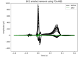
Principal Component Analysis - Optimal Basis Sets (PCA-OBS) removing cardiac artefact
Principal Component Analysis - Optimal Basis Sets (PCA-OBS) removing cardiac artefact
- get_montage()[source]#
Get a DigMontage from instance.
- Returns:
- montage
None|DigMontage A copy of the channel positions, if available, otherwise
None.
- montage
- get_peak(ch_type=None, tmin=None, tmax=None, mode='abs', time_as_index=False, merge_grads=False, return_amplitude=False, *, strict=True)[source]#
Get location and latency of peak amplitude.
- Parameters:
- ch_type
str|None The channel type to use. Defaults to None. If more than one channel type is present in the data, this value must be provided.
- tmin
float|None The minimum point in time to be considered for peak getting. If None (default), the beginning of the data is used.
- tmax
float|None The maximum point in time to be considered for peak getting. If None (default), the end of the data is used.
- mode‘pos’ | ‘neg’ | ‘abs’
How to deal with the sign of the data. If ‘pos’ only positive values will be considered. If ‘neg’ only negative values will be considered. If ‘abs’ absolute values will be considered. Defaults to ‘abs’.
- time_as_indexbool
Whether to return the time index instead of the latency in seconds.
- merge_gradsbool
If True, compute peak from merged gradiometer data.
- return_amplitudebool
If True, return also the amplitude at the maximum response.
New in v0.16.
- strictbool
If True, raise an error if values are all positive when detecting a minimum (mode=’neg’), or all negative when detecting a maximum (mode=’pos’). Defaults to True.
New in v1.7.
- ch_type
- Returns:
Examples using
get_peak:
- interpolate_bads(reset_bads=True, mode='accurate', origin='auto', method=None, exclude=(), on_bad_position='warn', verbose=None)[source]#
Interpolate bad MEG and EEG channels.
Operates in place.
- Parameters:
- reset_badsbool
If True, remove the bads from info.
- mode
str Either
'accurate'or'fast', determines the quality of the Legendre polynomial expansion used for interpolation of channels using the minimum-norm method.- originarray_like, shape (3,) |
str Origin of the sphere in the head coordinate frame and in meters. Can be
'auto'(default), which means a head-digitization-based origin fit.New in v0.17.
- method
dict|str|None Method to use for each channel type.
"meg"channels support"MNE"(default) and"nan""eeg"channels support"spline"(default),"MNE"and"nan""fnirs"channels support"nearest"(default) and"nan""ecog"channels support"spline"(default) and"nan""seeg"channels support"spline"(default) and"nan"
None is an alias for:
method=dict(meg="MNE", eeg="spline", fnirs="nearest")
If a
stris provided, the method will be applied to all channel types supported and available in the instance. The method"nan"will replace the channel data withnp.nan.Warning
Be careful when using
method="nan"; the default valuereset_bads=Truemay not be what you want.New in v0.21.
- exclude
list|tuple The channels to exclude from interpolation. If excluded a bad channel will stay in bads.
- on_bad_position“raise” | “warn” | “ignore”
What to do when one or more sensor positions are invalid (zero or NaN). If
"warn"or"ignore", channels with invalid positions will be filled withnan.New in v1.12.
- verbosebool |
str|int|None Control verbosity of the logging output. If
None, use the default verbosity level. See the logging documentation andmne.verbose()for details. Should only be passed as a keyword argument.
- Returns:
- instsame
typeas the input data The modified instance.
- instsame
Notes
The
"MNE"method uses minimum-norm projection to a sphere and back.New in v0.9.0.
- interpolate_to(sensors, origin='auto', method=None, mode='accurate', reg=0.0)[source]#
Interpolate data onto a new sensor configuration.
This method can interpolate EEG data onto a new montage or transform MEG data to a different sensor configuration (e.g., Neuromag to CTF).
- Parameters:
- sensors
DigMontage|str For EEG: A DigMontage object containing target channel positions. For MEG: A string specifying the target MEG system. Currently supported:
'neuromag','ctf151'or'ctf275'.- originarray_like, shape (3,) |
str Origin of the sphere in the head coordinate frame and in meters. Can be
'auto'(default), which means a head-digitization-based origin fit. Used for both EEG and MEG interpolation.- method
str|None Interpolation method to use. For EEG:
'spline'(default, same as None) or'MNE'. For MEG:'MNE'(default, same as None).Changed in version 1.10.0: Added support for MEG interpolation.
- mode
str Either
'accurate'(default) or'fast', determines the quality of the Legendre polynomial expansion used for interpolation of MEG channels using the minimum-norm method. Only used for MEG interpolation.- reg
float The regularization parameter for the interpolation method. Only used when
method='spline'for EEG channels.
- sensors
- Returns:
- instsame
typeas the input data A new instance with interpolated data and updated channel information.
- instsame
Notes
For EEG data:
This method interpolates EEG channels onto a new montage using spherical splines or minimum-norm estimation. Non-EEG channels are preserved without modification.
For MEG data:
This method transforms MEG data to a different sensor configuration using field interpolation.
Common use cases for MEG transformation:
Transform Neuromag data to CTF sensor layout for comparison
Transform CTF data to Neuromag sensor layout
Simulate what data would look like on a different MEG system
Warning
MEG field interpolation assumes that the head position relative to the sensors is similar between systems. Large differences in head position may affect interpolation accuracy.
New in v1.10.0.
Changed in version 1.12.0: Added support for MEG interpolation to canonical systems.
- property kind#
The data kind.
- pick(picks, exclude=(), *, verbose=None)[source]#
Pick a subset of channels.
- Parameters:
- picks
str| array_like |slice|None Channels to include. Slices and lists of integers will be interpreted as channel indices. In lists, channel type strings (e.g.,
['meg',
'eeg']
) will pick channels of those types, channel name strings (e.g.,['MEG0111', 'MEG2623']will pick the given channels. Can also be the string values'all'to pick all channels, or'data'to pick data channels. None (default) will pick all channels. Bad channels are included by default. Note that channels ininfo['bads']will be included if their names or indices are explicitly provided.- exclude
list|str Set of channels to exclude, only used when picking based on types (e.g., exclude=”bads” when picks=”meg”).
- verbosebool |
str|int|None Control verbosity of the logging output. If
None, use the default verbosity level. See the logging documentation andmne.verbose()for details. Should only be passed as a keyword argument.New in v0.24.0.
- picks
- Returns:
- instsame
typeas the input data The modified instance.
- instsame
Examples using
pick:
Compute a sparse inverse solution using the Gamma-MAP empirical Bayesian method
Compute a sparse inverse solution using the Gamma-MAP empirical Bayesian method
Compute sparse inverse solution with mixed norm: MxNE and irMxNE
Compute sparse inverse solution with mixed norm: MxNE and irMxNE
Computing source timecourses with an XFit-like multi-dipole model
Computing source timecourses with an XFit-like multi-dipole model
Source localization with equivalent current dipole (ECD) fit
Source localization with equivalent current dipole (ECD) fit
- pick_channels(ch_names, ordered=True, *, verbose=None)[source]#
Warning
LEGACY: New code should use inst.pick(…).
Pick some channels.
- Parameters:
- ch_names
list The list of channels to select.
- orderedbool
If True (default), ensure that the order of the channels in the modified instance matches the order of
ch_names.New in v0.20.0.
Changed in version 1.7: The default changed from False in 1.6 to True in 1.7.
- verbosebool |
str|int|None Control verbosity of the logging output. If
None, use the default verbosity level. See the logging documentation andmne.verbose()for details. Should only be passed as a keyword argument.New in v1.1.
- ch_names
- Returns:
- instsame
typeas the input data The modified instance.
- instsame
See also
Notes
If
orderedisFalse, the channel names given viach_namesare assumed to be a set, that is, their order does not matter. In that case, the original order of the channels in the data is preserved. Apart from usingordered=True, you may also usereorder_channelsto set channel order, if necessary.New in v0.9.0.
Examples using
pick_channels:
- pick_types(meg=False, eeg=False, stim=False, eog=False, ecg=False, emg=False, ref_meg='auto', *, misc=False, resp=False, chpi=False, exci=False, ias=False, syst=False, seeg=False, dipole=False, gof=False, bio=False, ecog=False, fnirs=False, csd=False, dbs=False, temperature=False, gsr=False, eyetrack=False, include=(), exclude='bads', selection=None, verbose=None)[source]#
Warning
LEGACY: New code should use inst.pick(…).
Pick some channels by type and names.
- Parameters:
- megbool |
str If True include MEG channels. If string it can be ‘mag’, ‘grad’, ‘planar1’ or ‘planar2’ to select only magnetometers, all gradiometers, or a specific type of gradiometer.
- eegbool
If True include EEG channels.
- stimbool
If True include stimulus channels.
- eogbool
If True include EOG channels.
- ecgbool
If True include ECG channels.
- emgbool
If True include EMG channels.
- ref_megbool |
str If True include CTF / 4D reference channels. If ‘auto’, reference channels are included if compensations are present and
megis not False. Can also be the string options for themegparameter.- miscbool
If True include miscellaneous analog channels.
- respbool
If
Trueinclude respiratory channels.- chpibool
If True include continuous HPI coil channels.
- excibool
Flux excitation channel used to be a stimulus channel.
- iasbool
Internal Active Shielding data (maybe on Triux only).
- systbool
System status channel information (on Triux systems only).
- seegbool
Stereotactic EEG channels.
- dipolebool
Dipole time course channels.
- gofbool
Dipole goodness of fit channels.
- biobool
Bio channels.
- ecogbool
Electrocorticography channels.
- fnirsbool |
str Functional near-infrared spectroscopy channels. If True include all fNIRS channels. If False (default) include none. If string it can be ‘hbo’ (to include channels measuring oxyhemoglobin) or ‘hbr’ (to include channels measuring deoxyhemoglobin).
- csdbool
EEG-CSD channels.
- dbsbool
Deep brain stimulation channels.
- temperaturebool
Temperature channels.
- gsrbool
Galvanic skin response channels.
- eyetrackbool |
str Eyetracking channels. If True include all eyetracking channels. If False (default) include none. If string it can be ‘eyegaze’ (to include eye position channels) or ‘pupil’ (to include pupil-size channels).
- include
listofstr List of additional channels to include. If empty do not include any.
- exclude
listofstr|str List of channels to exclude. If ‘bads’ (default), exclude channels in
info['bads'].- selection
listofstr Restrict sensor channels (MEG, EEG, etc.) to this list of channel names.
- verbosebool |
str|int|None Control verbosity of the logging output. If
None, use the default verbosity level. See the logging documentation andmne.verbose()for details. Should only be passed as a keyword argument.
- megbool |
- Returns:
- instsame
typeas the input data The modified instance.
- instsame
See also
Notes
New in v0.9.0.
- plot(picks=None, exclude='bads', unit=True, show=True, ylim=None, xlim='tight', proj=False, hline=None, units=None, scalings=None, titles=None, axes=None, gfp=False, window_title=None, spatial_colors='auto', zorder='unsorted', selectable=True, noise_cov=None, time_unit='s', sphere=None, *, highlight=None, verbose=None)[source]#
Plot evoked data using butterfly plots.
Left click to a line shows the channel name. Selecting an area by clicking and holding left mouse button plots a topographic map of the painted area.
Note
If bad channels are not excluded they are shown in red.
- Parameters:
- picks
str| array_like |slice|None Channels to include. Slices and lists of integers will be interpreted as channel indices. In lists, channel type strings (e.g.,
['meg',
'eeg']
) will pick channels of those types, channel name strings (e.g.,['MEG0111', 'MEG2623']will pick the given channels. Can also be the string values'all'to pick all channels, or'data'to pick data channels. None (default) will pick all channels. Bad channels are included by default. Note that channels ininfo['bads']will be included if their names or indices are explicitly provided.- exclude
listofstr|'bads' Channels names to exclude from being shown. If
'bads', the bad channels are excluded.- unitbool
Scale plot with channel (SI) unit.
- showbool
Show figure if True.
- ylim
dict|None Y-axis limits for plots (after scaling has been applied).
dictkeys should match channel types; valid keys are for instanceeeg,mag,grad,misc,csd, .. (example:ylim=dict(eeg=[-20, 20])). IfNone, the y-axis limits will be set automatically by matplotlib. Defaults toNone.- xlim
'tight'|tuple|None Limits for the X-axis of the plots.
- projbool | ‘interactive’ | ‘reconstruct’
If true SSP projections are applied before display. If
'interactive', a check box for reversible selection of SSP projection vectors will be shown. If'reconstruct', projection vectors will be applied and then M/EEG data will be reconstructed via field mapping to reduce the signal bias caused by projection.Changed in version 0.21: Support for ‘reconstruct’ was added.
- hline
listoffloat|None The values at which to show an horizontal line.
- units
dict|None The units of the channel types used for axes labels. If None, defaults to
dict(eeg='µV', grad='fT/cm', mag='fT').- scalings
dict|None The scalings of the channel types to be applied for plotting. If None, defaults to
dict(eeg=1e6, grad=1e13, mag=1e15).- titles
dict|None The titles associated with the channels. If None, defaults to
dict(eeg='EEG', grad='Gradiometers', mag='Magnetometers').- axesinstance of
Axes|list|None The axes to plot to. If list, the list must be a list of Axes of the same length as the number of channel types. If instance of Axes, there must be only one channel type plotted.
- gfpbool |
'only' Plot the global field power (GFP) or the root mean square (RMS) of the data. For MEG data, this will plot the RMS. For EEG, it plots GFP, i.e. the standard deviation of the signal across channels. The GFP is equivalent to the RMS of an average-referenced signal.
TruePlot GFP or RMS (for EEG and MEG, respectively) and traces for all channels.
'only'Plot GFP or RMS (for EEG and MEG, respectively), and omit the traces for individual channels.
The color of the GFP/RMS trace will be green if
spatial_colors=False, and black otherwise.Changed in version 0.23: Plot GFP for EEG instead of RMS. Label RMS traces correctly as such.
- window_title
str|None The title to put at the top of the figure.
- spatial_colorsbool | ‘auto’
If True, the lines are color coded by mapping physical sensor coordinates into color values. Spatially similar channels will have similar colors. Bad channels will be dotted. If False, the good channels are plotted black and bad channels red. If
'auto', uses True if channel locations are present, and False if channel locations are missing or if the data contains only a single channel. Defaults to'auto'.- zorder
str|callable() Which channels to put in the front or back. Only matters if
spatial_colorsis used. If str, must bestdorunsorted(defaults tounsorted). Ifstd, data with the lowest standard deviation (weakest effects) will be put in front so that they are not obscured by those with stronger effects. Ifunsorted, channels are z-sorted as in the evoked instance. If callable, must take one argument: a numpy array of the same dimensionality as the evoked raw data; and return a list of unique integers corresponding to the number of channels.New in v0.13.0.
- selectablebool
Whether to use interactive features. If True (default), it is possible to paint an area to draw topomaps. When False, the interactive features are disabled. Disabling interactive features reduces memory consumption and is useful when using
axesparameter to draw multiaxes figures.New in v0.13.0.
- noise_covinstance of
Covariance|str|None Noise covariance used to whiten the data while plotting. Whitened data channel names are shown in italic. Can be a string to load a covariance from disk. See also
mne.Evoked.plot_white()for additional inspection of noise covariance properties when whitening evoked data. For data processed with SSS, the effective dependence between magnetometers and gradiometers may introduce differences in scaling, consider usingmne.Evoked.plot_white().New in v0.16.0.
- time_unit
str The units for the time axis, can be “s” (default) or “ms”.
New in v0.16.
- sphere
float| array_like offloat| instance ofConductorModel|str|listofstr|None The sphere parameters to use for the head outline. Can be array-like of shape (4,) to give the X/Y/Z origin and radius in meters, or a single float to give just the radius (origin assumed 0, 0, 0). Can also be an instance of a spherical
ConductorModelto use the origin and radius from that object. Can also be astr, in which case:'auto': the sphere is fit to external digitization points first, and to external + EEG digitization points if the former fails.'eeglab': the head circle is defined by EEG electrodes'Fpz','Oz','T7', and'T8'(if'Fpz'is not present, it will be approximated from the coordinates of'Oz').'extra': the sphere is fit to external digitization points.'eeg': the sphere is fit to EEG digitization points.'cardinal': the sphere is fit to cardinal digitization points.'hpi': the sphere is fit to HPI coil digitization points.
Can also be a list of
str, in which case the sphere is fit to the specified digitization points, which can be any combination of'extra','eeg','cardinal', and'hpi', as specified above.None(the default) is equivalent to'auto'when enough extra digitization points are available, and (0, 0, 0, 0.095) otherwise.New in v0.20.
Changed in version 1.1: Added
'eeglab'option.Changed in version 1.11: Added
'extra','eeg','cardinal','hpi'and list ofstroptions.- highlightarray_like of
float, shape(2,) | array_like offloat, shape (n, 2) |None Segments of the data to highlight by means of a light-yellow background color. Can be used to put visual emphasis on certain time periods. The time periods must be specified as
array-likeobjects in the form of(t_start, t_end)in the unit given by thetime_unitparameter. Multiple time periods can be specified by passing anarray-likeobject of individual time periods (e.g., for 3 time periods, the shape of the passed object would be(3, 2). IfNone, no highlighting is applied.New in v1.1.
- verbosebool |
str|int|None Control verbosity of the logging output. If
None, use the default verbosity level. See the logging documentation andmne.verbose()for details. Should only be passed as a keyword argument.
- picks
- Returns:
- figinstance of
matplotlib.figure.Figure Figure containing the butterfly plots.
- figinstance of
See also
Examples using
plot:
Analysis of evoked response using ICA and PCA reduction techniques
Analysis of evoked response using ICA and PCA reduction techniques
Compute a sparse inverse solution using the Gamma-MAP empirical Bayesian method
Compute a sparse inverse solution using the Gamma-MAP empirical Bayesian method
Compute sparse inverse solution with mixed norm: MxNE and irMxNE
Compute sparse inverse solution with mixed norm: MxNE and irMxNE
Compute source power estimate by projecting the covariance with MNE
Compute source power estimate by projecting the covariance with MNE
Define target events based on time lag, plot evoked response
Define target events based on time lag, plot evoked response
Source localization with MNE, dSPM, sLORETA, and eLORETA
Source localization with MNE, dSPM, sLORETA, and eLORETA
Working with CTF data: the Brainstorm auditory dataset
Working with CTF data: the Brainstorm auditory dataset
Non-parametric 1 sample cluster statistic on single trial power
Non-parametric 1 sample cluster statistic on single trial power
Non-parametric between conditions cluster statistic on single trial power
Non-parametric between conditions cluster statistic on single trial power
- plot_field(surf_maps, time=None, time_label='t = %0.0f ms', n_jobs=None, fig=None, vmax=None, n_contours=21, *, show_density=True, alpha=None, interpolation='nearest', interaction='terrain', time_viewer='auto', verbose=None)[source]#
Plot MEG/EEG fields on head surface and helmet in 3D.
- Parameters:
- surf_maps
list The surface mapping information obtained with make_field_map.
- time
float|None The time point at which the field map shall be displayed. If None, the average peak latency (across sensor types) is used.
- time_label
str|None How to print info about the time instant visualized.
- n_jobs
int|None The number of jobs to run in parallel. If
-1, it is set to the number of CPU cores. Requires thejoblibpackage.None(default) is a marker for ‘unset’ that will be interpreted asn_jobs=1(sequential execution) unless the call is performed under ajoblib.parallel_configcontext manager that sets another value forn_jobs.- fig
Figure3D|mne.viz.Brain|None If None (default), a new figure will be created, otherwise it will plot into the given figure.
New in v0.20.
New in v1.4:
figcan also be aBrainfigure.- vmax
float|dict|None Maximum intensity. Can be a dictionary with two entries
"eeg"and"meg"to specify separate values for EEG and MEG fields respectively. Can beNoneto use the maximum value of the data.New in v0.21.
New in v1.4:
vmaxcan be a dictionary to specify separate values for EEG and MEG fields.- n_contours
int The number of contours.
New in v0.21.
- show_densitybool
Whether to draw the field density as an overlay on top of the helmet/head surface. Defaults to
True.New in v1.6.
- alpha
float|dict|None Opacity of the meshes (between 0 and 1). Can be a dictionary with two entries
"eeg"and"meg"to specify separate values for EEG and MEG fields respectively. Can beNoneto use 1.0 when a single field map is shown, ordict(eeg=1.0, meg=0.5)when both field maps are shown.New in v1.4.
- interpolation
str|None Interpolation method (
scipy.interpolate.interp1dparameter). Must be one of'linear','nearest','zero','slinear','quadratic'or'cubic'.New in v1.6.
- interaction‘trackball’ | ‘terrain’
How interactions with the scene via an input device (e.g., mouse or trackpad) modify the camera position. If
'terrain', one axis is fixed, enabling “turntable-style” rotations. If'trackball', movement along all axes is possible, which provides more freedom of movement, but you may incidentally perform unintentional rotations along some axes. Defaults to'terrain'.New in v1.1.
- time_viewerbool |
str Display time viewer GUI. Can also be
"auto", which will meanTrueif there is more than one time point andFalseotherwise.New in v1.6.
- verbosebool |
str|int|None Control verbosity of the logging output. If
None, use the default verbosity level. See the logging documentation andmne.verbose()for details. Should only be passed as a keyword argument.
- surf_maps
- Returns:
- fig
Figure3D|mne.viz.EvokedField Without the time viewer active, the figure is returned. With the time viewer active, an object is returned that can be used to control different aspects of the figure.
- fig
Examples using
plot_field:
- plot_image(picks=None, exclude='bads', unit=True, show=True, clim=None, xlim='tight', proj=False, units=None, scalings=None, titles=None, axes=None, cmap='RdBu_r', colorbar=True, mask=None, mask_style=None, mask_cmap='Greys', mask_alpha=0.25, time_unit='s', show_names=None, group_by=None, sphere=None)[source]#
Plot evoked data as images.
- Parameters:
- picks
str| array_like |slice|None Channels to include. Slices and lists of integers will be interpreted as channel indices. In lists, channel type strings (e.g.,
['meg',
'eeg']
) will pick channels of those types, channel name strings (e.g.,['MEG0111', 'MEG2623']will pick the given channels. Can also be the string values'all'to pick all channels, or'data'to pick data channels. None (default) will pick all channels. Bad channels are included by default. Note that channels ininfo['bads']will be included if their names or indices are explicitly provided. This parameter can also be used to set the order the channels are shown in, as the channel image is sorted by the order of picks.- exclude
listofstr| ‘bads’ Channels names to exclude from being shown. If ‘bads’, the bad channels are excluded.
- unitbool
Scale plot with channel (SI) unit.
- showbool
Show figure if True.
- clim
dict|None Color limits for plots (after scaling has been applied). e.g.
clim = dict(eeg=[-20, 20]). Valid keys are eeg, mag, grad, misc. If None, the clim parameter for each channel equals the pyplot default.- xlim‘tight’ |
tuple|None X limits for plots.
- projbool | ‘interactive’
If true SSP projections are applied before display. If ‘interactive’, a check box for reversible selection of SSP projection vectors will be shown.
- units
dict|None The units of the channel types used for axes labels. If None, defaults to
dict(eeg='µV', grad='fT/cm', mag='fT').- scalings
dict|None The scalings of the channel types to be applied for plotting. If None,` defaults to
dict(eeg=1e6, grad=1e13, mag=1e15).- titles
dict|None The titles associated with the channels. If None, defaults to
dict(eeg='EEG', grad='Gradiometers', mag='Magnetometers').- axesinstance of
Axes|list|dict|None The axes to plot to. If list, the list must be a list of Axes of the same length as the number of channel types. If instance of Axes, there must be only one channel type plotted. If
group_byis a dict, this cannot be a list, but it can be a dict of lists of axes, with the keys matching those ofgroup_by. In that case, the provided axes will be used for the corresponding groups. Defaults toNone.- cmapmatplotlib colormap | (colormap, bool) | ‘interactive’
Colormap. If tuple, the first value indicates the colormap to use and the second value is a boolean defining interactivity. In interactive mode the colors are adjustable by clicking and dragging the colorbar with left and right mouse button. Left mouse button moves the scale up and down and right mouse button adjusts the range. Hitting space bar resets the scale. Up and down arrows can be used to change the colormap. If ‘interactive’, translates to
('RdBu_r', True). Defaults to'RdBu_r'.- colorbarbool
If True, plot a colorbar. Defaults to True.
New in v0.16.
- mask
ndarray|None An array of booleans of the same shape as the data. Entries of the data that correspond to
Falsein the mask are masked (seedo_maskbelow). Useful for, e.g., masking for statistical significance.New in v0.16.
- mask_style
None| ‘both’ | ‘contour’ | ‘mask’ If
maskis not None: if ‘contour’, a contour line is drawn around the masked areas (Trueinmask). If ‘mask’, entries notTrueinmaskare shown transparently. If ‘both’, both a contour and transparency are used. IfNone, defaults to ‘both’ ifmaskis not None, and is ignored otherwise.New in v0.16.
- mask_cmapmatplotlib colormap | (colormap, bool) | ‘interactive’
The colormap chosen for masked parts of the image (see below), if
maskis notNone. If None,cmapis reused. Defaults toGreys. Not interactive. Otherwise, ascmap.- mask_alpha
float A float between 0 and 1. If
maskis not None, this sets the alpha level (degree of transparency) for the masked-out segments. I.e., if 0, masked-out segments are not visible at all. Defaults to .25.New in v0.16.
- time_unit
str The units for the time axis, can be “ms” or “s” (default).
New in v0.16.
- show_namesbool | ‘auto’ | ‘all’
Determines if channel names should be plotted on the y axis. If False, no names are shown. If True, ticks are set automatically by matplotlib and the corresponding channel names are shown. If “all”, all channel names are shown. If “auto”, is set to False if
picksisNone, toTrueifpickscontains 25 or more entries, or to “all” ifpickscontains fewer than 25 entries.- group_by
None|dict If a dict, the values must be picks, and
axesmust also be a dict with matching keys, or None. Ifaxesis None, one figure and one axis will be created for each entry ingroup_by.Then, for each entry, the picked channels will be plotted to the corresponding axis. Iftitlesare None, keys will become plot titles. This is useful for e.g. ROIs. Each entry must contain only one channel type. For example:group_by=dict(Left_ROI=[1, 2, 3, 4], Right_ROI=[5, 6, 7, 8])
If None, all picked channels are plotted to the same axis.
- sphere
float| array_like offloat| instance ofConductorModel|str|listofstr|None The sphere parameters to use for the head outline. Can be array-like of shape (4,) to give the X/Y/Z origin and radius in meters, or a single float to give just the radius (origin assumed 0, 0, 0). Can also be an instance of a spherical
ConductorModelto use the origin and radius from that object. Can also be astr, in which case:'auto': the sphere is fit to external digitization points first, and to external + EEG digitization points if the former fails.'eeglab': the head circle is defined by EEG electrodes'Fpz','Oz','T7', and'T8'(if'Fpz'is not present, it will be approximated from the coordinates of'Oz').'extra': the sphere is fit to external digitization points.'eeg': the sphere is fit to EEG digitization points.'cardinal': the sphere is fit to cardinal digitization points.'hpi': the sphere is fit to HPI coil digitization points.
Can also be a list of
str, in which case the sphere is fit to the specified digitization points, which can be any combination of'extra','eeg','cardinal', and'hpi', as specified above.None(the default) is equivalent to'auto'when enough extra digitization points are available, and (0, 0, 0, 0.095) otherwise.New in v0.20.
Changed in version 1.1: Added
'eeglab'option.Changed in version 1.11: Added
'extra','eeg','cardinal','hpi'and list ofstroptions.
- picks
- Returns:
- figinstance of
matplotlib.figure.Figure Figure containing the images.
- figinstance of
Examples using
plot_image:
Analysing continuous features with binning and regression in sensor space
Analysing continuous features with binning and regression in sensor space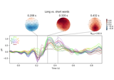
Visualising statistical significance thresholds on EEG data
Visualising statistical significance thresholds on EEG data
- plot_joint(times='peaks', title='', picks=None, exclude='bads', show=True, ts_args=None, topomap_args=None)[source]#
Plot evoked data as butterfly plot and add topomaps for time points.
Note
Axes to plot in can be passed by the user through
ts_argsortopomap_args. In that case bothts_argsandtopomap_argsaxes have to be used. Be aware that when the axes are provided, their position may be slightly modified.- Parameters:
- times
float|arrayoffloat| “auto” | “peaks” The time point(s) to plot. If
"auto", 5 evenly spaced topographies between the first and last time instant will be shown. If"peaks", finds time points automatically by checking for 3 local maxima in Global Field Power. Defaults to"peaks".- title
str|None The title. If
None, suppress printing channel type title. If an empty string, a default title is created. Defaults to ‘’. If custom axes are passed make sure to settitle=None, otherwise some of your axes may be removed during placement of the title axis.- picks
str| array_like |slice|None Channels to include. Slices and lists of integers will be interpreted as channel indices. In lists, channel type strings (e.g.,
['meg',
'eeg']
) will pick channels of those types, channel name strings (e.g.,['MEG0111', 'MEG2623']will pick the given channels. Can also be the string values'all'to pick all channels, or'data'to pick data channels. None (default) will pick all channels. Bad channels are included by default. Note that channels ininfo['bads']will be included if their names or indices are explicitly provided.- exclude
listofstr| ‘bads’ Channels names to exclude from being shown. If
'bads', the bad channels are excluded. Defaults to'bads'.- showbool
Show figure if
True. Defaults toTrue.- ts_args
None|dict A dict of
kwargsthat are forwarded tomne.Evoked.plot()to style the butterfly plot. If they are not in this dict, the following defaults are passed:spatial_colors=True,zorder='std'.showandexcludeare illegal. IfNone, no customizable arguments will be passed. Defaults toNone.- topomap_args
None|dict A dict of
kwargsthat are forwarded tomne.Evoked.plot_topomap()to style the topomaps. If it is not in this dict,outlines='head'will be passed.show,times,colorbarare illegal. IfNone, no customizable arguments will be passed. Defaults toNone.
- times
- Returns:
- figinstance of
matplotlib.figure.Figure|list The figure object containing the plot. If
evokedhas multiple channel types, a list of figures, one for each channel type, is returned.
- figinstance of
Notes
New in v0.12.0.
Examples using
plot_joint: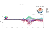
Single trial linear regression analysis with the LIMO dataset
Single trial linear regression analysis with the LIMO dataset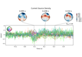
Transform EEG data using current source density (CSD)
Transform EEG data using current source density (CSD)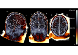
EEG source localization given electrode locations on an MRI
EEG source localization given electrode locations on an MRI
Preprocessing optically pumped magnetometer (OPM) MEG data
Preprocessing optically pumped magnetometer (OPM) MEG data
Visualising statistical significance thresholds on EEG data
Visualising statistical significance thresholds on EEG data
- plot_projs_topomap(ch_type=None, *, sensors=True, show_names=False, contours=6, outlines='head', sphere=None, image_interp='cubic', extrapolate='auto', border='mean', res=64, size=1, cmap=None, vlim=(None, None), cnorm=None, colorbar=False, cbar_fmt='%3.1f', units=None, axes=None, show=True)[source]#
Plot SSP vector.
- Parameters:
- ch_type‘mag’ | ‘grad’ | ‘planar1’ | ‘planar2’ | ‘eeg’ |
None|list The channel type to plot. For
'grad', the gradiometers are collected in pairs and the RMS for each pair is plotted. IfNoneit will return all channel types present.. If a list of ch_types is provided, it will return multiple figures. Defaults toNone.- sensorsbool |
str Whether to add markers for sensor locations. If
str, should be a valid matplotlib format string (e.g.,'r+'for red plusses, see the Notes section ofplot()). IfTrue(the default), black circles will be used.- show_namesbool |
callable() If
True, show channel names next to each sensor marker. If callable, channel names will be formatted using the callable; e.g., to delete the prefix ‘MEG ‘ from all channel names, pass the functionlambda x: x.replace('MEG ', ''). Ifmaskis notNone, only non-masked sensor names will be shown.New in v1.2.
- contours
int| array_like The number of contour lines to draw. If
0, no contours will be drawn. If a positive integer, that number of contour levels are chosen using the matplotlib tick locator (may sometimes be inaccurate, use array for accuracy). If array-like, the array values are used as the contour levels. The values should be in µV for EEG, fT for magnetometers and fT/m for gradiometers. Ifcolorbar=True, the colorbar will have ticks corresponding to the contour levels. Default is6.- outlines‘head’ |
dict|None The outlines to be drawn. If ‘head’, the default head scheme will be drawn. If dict, each key refers to a tuple of x and y positions, the values in ‘mask_pos’ will serve as image mask. Alternatively, a matplotlib patch object can be passed for advanced masking options, either directly or as a function that returns patches (required for multi-axis plots). If None, nothing will be drawn. Defaults to ‘head’.
- sphere
float| array_like offloat| instance ofConductorModel|str|listofstr|None The sphere parameters to use for the head outline. Can be array-like of shape (4,) to give the X/Y/Z origin and radius in meters, or a single float to give just the radius (origin assumed 0, 0, 0). Can also be an instance of a spherical
ConductorModelto use the origin and radius from that object. Can also be astr, in which case:'auto': the sphere is fit to external digitization points first, and to external + EEG digitization points if the former fails.'eeglab': the head circle is defined by EEG electrodes'Fpz','Oz','T7', and'T8'(if'Fpz'is not present, it will be approximated from the coordinates of'Oz').'extra': the sphere is fit to external digitization points.'eeg': the sphere is fit to EEG digitization points.'cardinal': the sphere is fit to cardinal digitization points.'hpi': the sphere is fit to HPI coil digitization points.
Can also be a list of
str, in which case the sphere is fit to the specified digitization points, which can be any combination of'extra','eeg','cardinal', and'hpi', as specified above.None(the default) is equivalent to'auto'when enough extra digitization points are available, and (0, 0, 0, 0.095) otherwise.New in v0.20.
Changed in version 1.1: Added
'eeglab'option.Changed in version 1.11: Added
'extra','eeg','cardinal','hpi'and list ofstroptions.- image_interp
str The image interpolation to be used. Options are
'cubic'(default) to usescipy.interpolate.CloughTocher2DInterpolator,'nearest'to usescipy.spatial.Voronoior'linear'to usescipy.interpolate.LinearNDInterpolator.- extrapolate
str Options:
'box'Extrapolate to four points placed to form a square encompassing all data points, where each side of the square is three times the range of the data in the respective dimension.
'local'(default for MEG sensors)Extrapolate only to nearby points (approximately to points closer than median inter-electrode distance). This will also set the mask to be polygonal based on the convex hull of the sensors.
'head'(default for non-MEG sensors)Extrapolate out to the edges of the clipping circle. This will be on the head circle when the sensors are contained within the head circle, but it can extend beyond the head when sensors are plotted outside the head circle.
New in v0.20.
Changed in version 0.21:
The default was changed to
'local'for MEG sensors.'local'was changed to use a convex hull mask'head'was changed to extrapolate out to the clipping circle.
- border
float| ‘mean’ Value to extrapolate to on the topomap borders. If
'mean'(default), then each extrapolated point has the average value of its neighbours.New in v0.20.
- res
int The resolution of the topomap image (number of pixels along each side).
- size
float Side length of each subplot in inches. Only applies when plotting multiple topomaps at a time.
- cmapmatplotlib colormap | (colormap, bool) | ‘interactive’ |
None Colormap to use. If
tuple, the first value indicates the colormap to use and the second value is a boolean defining interactivity. In interactive mode the colors are adjustable by clicking and dragging the colorbar with left and right mouse button. Left mouse button moves the scale up and down and right mouse button adjusts the range. Hitting space bar resets the range. Up and down arrows can be used to change the colormap. IfNone,'Reds'is used for data that is either all-positive or all-negative, and'RdBu_r'is used otherwise.'interactive'is equivalent to(None, True). Defaults toNone.Warning
Interactive mode works smoothly only for a small amount of topomaps. Interactive mode is disabled by default for more than 2 topomaps.
- vlim
tupleof length 2 | “joint” Lower and upper bounds of the colormap, typically a numeric value in the same units as the data. Elements of the
tuplemay also be callable functions which take in aNumPy arrayand return a scalar.If both entries are
None, the bounds are set at ± the maximum absolute value of the data (yielding a colormap with midpoint at 0), or(0, max(abs(data)))if the (possibly baselined) data are all-positive. ProvidingNonefor just one entry will set the corresponding boundary at the min/max of the data. Ifvlim="joint", will compute the colormap limits jointly across all projectors of the same channel type (instead of separately for each projector), using the min/max of the data for that channel type. If vlim is"joint",infomust not beNone. Defaults to(None, None).- cnorm
matplotlib.colors.Normalize|None How to normalize the colormap. If
None, standard linear normalization is performed. If notNone,vminandvmaxwill be ignored. See Matplotlib docs for more details on colormap normalization, and the ERDs example for an example of its use.New in v1.2.
- colorbarbool
Plot a colorbar in the rightmost column of the figure.
- cbar_fmt
str Formatting string for colorbar tick labels. See Format specification mini-language for details.
New in v1.2.
- units
str|None The units to use for the colorbar label. Ignored if
colorbar=False. IfNonethe label will be “AU” indicating arbitrary units. Default isNone.New in v1.2.
- axesinstance of
Axes|listofAxes|None The axes to plot into. If
None, a newFigurewill be created with the correct number of axes. IfAxesare provided (either as a single instance or alistof axes), the number of axes provided must match the number of projectors. Default isNone.- showbool
Show the figure if
True.
- ch_type‘mag’ | ‘grad’ | ‘planar1’ | ‘planar2’ | ‘eeg’ |
- Returns:
- figinstance of
Figure Figure distributing one image per channel across sensor topography.
- figinstance of
- plot_psd(fmin=0, fmax=inf, tmin=None, tmax=None, picks=None, proj=False, *, method='auto', average=False, dB=True, estimate='power', xscale='linear', area_mode='std', area_alpha=0.33, color='black', line_alpha=None, spatial_colors=True, sphere=None, exclude='bads', ax=None, show=True, n_jobs=1, verbose=None, **method_kw)[source]#
Plot power or amplitude spectra.
Separate plots are drawn for each channel type. When the data have been processed with a bandpass, lowpass or highpass filter, dashed lines (╎) indicate the boundaries of the filter. The line noise frequency is also indicated with a dashed line (⋮). If
average=False, the plot will be interactive, and click-dragging on the spectrum will generate a scalp topography plot for the chosen frequency range in a new figure.- Parameters:
- fmin, fmax
float The lower- and upper-bound on frequencies of interest. Default is
fmin=0, fmax=np.inf(spans all frequencies present in the data).- tmin, tmax
float|None First and last times to include, in seconds.
Noneuses the first or last time present in the data. Default istmin=None, tmax=None(all times).- picks
str| array_like |slice|None Channels to include. Slices and lists of integers will be interpreted as channel indices. In lists, channel type strings (e.g.,
['meg',
'eeg']
) will pick channels of those types, channel name strings (e.g.,['MEG0111', 'MEG2623']will pick the given channels. Can also be the string values'all'to pick all channels, or'data'to pick data channels. None (default) will pick good data channels (excluding reference MEG channels). Note that channels ininfo['bads']will be included if their names or indices are explicitly provided.- projbool
Whether to apply SSP projection vectors before spectral estimation. Default is
False.- method
'welch'|'multitaper'|'auto' Spectral estimation method.
'welch'uses Welch’s method [1],'multitaper'uses DPSS tapers [2].'auto'(default) uses Welch’s method for continuous data and multitaper forEpochsorEvokeddata.- averagebool
If False, the PSDs of all channels is displayed. No averaging is done and parameters area_mode and area_alpha are ignored. When False, it is possible to paint an area (hold left mouse button and drag) to plot a topomap.
- dBbool
Plot power spectral density (PSD) in units (dB/Hz) if
dB=Trueandestimate='power'. Plot PSD in units (amplitude**2/Hz) ifdB=Falseandestimate='power'. Plot amplitude spectral density (ASD) in units (amplitude/sqrt(Hz)) ifdB=Falseandestimate='amplitude'. Plot ASD in units (dB/sqrt(Hz)) ifdB=Trueandestimate='amplitude'.- estimate
str, {‘power’, ‘amplitude’} Can be “power” for power spectral density (PSD; default), “amplitude” for amplitude spectrum density (ASD).
- xscale‘linear’ | ‘log’
Scale of the frequency axis. Default is
'linear'.- area_mode
str|None Mode for plotting area. If ‘std’, the mean +/- 1 STD (across channels) will be plotted. If ‘range’, the min and max (across channels) will be plotted. Bad channels will be excluded from these calculations. If None, no area will be plotted. If average=False, no area is plotted.
- area_alpha
float Alpha for the area.
- color
str|tuple A matplotlib-compatible color to use. Has no effect when spatial_colors=True.
- line_alpha
float|None Alpha for the PSD line. Can be None (default) to use 1.0 when
average=Trueand 0.1 whenaverage=False.- spatial_colorsbool
Whether to color spectrum lines by channel location. Ignored if
average=True.- sphere
float| array_like offloat| instance ofConductorModel|str|listofstr|None The sphere parameters to use for the head outline. Can be array-like of shape (4,) to give the X/Y/Z origin and radius in meters, or a single float to give just the radius (origin assumed 0, 0, 0). Can also be an instance of a spherical
ConductorModelto use the origin and radius from that object. Can also be astr, in which case:'auto': the sphere is fit to external digitization points first, and to external + EEG digitization points if the former fails.'eeglab': the head circle is defined by EEG electrodes'Fpz','Oz','T7', and'T8'(if'Fpz'is not present, it will be approximated from the coordinates of'Oz').'extra': the sphere is fit to external digitization points.'eeg': the sphere is fit to EEG digitization points.'cardinal': the sphere is fit to cardinal digitization points.'hpi': the sphere is fit to HPI coil digitization points.
Can also be a list of
str, in which case the sphere is fit to the specified digitization points, which can be any combination of'extra','eeg','cardinal', and'hpi', as specified above.None(the default) is equivalent to'auto'when enough extra digitization points are available, and (0, 0, 0, 0.095) otherwise.New in v0.20.
Changed in version 1.1: Added
'eeglab'option.Changed in version 1.11: Added
'extra','eeg','cardinal','hpi'and list ofstroptions.New in v0.22.0.
- exclude
listofstr| ‘bads’ Channels names to exclude from being shown. If ‘bads’, the bad channels are excluded. Pass an empty list to plot all channels (including channels marked “bad”, if any).
New in v0.24.0.
- axinstance of
Axes|listofAxes|None The axes to plot into. If
None, a newFigurewill be created with the correct number of axes. IfAxesare provided (either as a single instance or alistof axes), the number of axes provided must match the number of channel types present in the object.. Default isNone.- showbool
Show the figure if
True.- n_jobs
int|None The number of jobs to run in parallel. If
-1, it is set to the number of CPU cores. Requires thejoblibpackage.None(default) is a marker for ‘unset’ that will be interpreted asn_jobs=1(sequential execution) unless the call is performed under ajoblib.parallel_configcontext manager that sets another value forn_jobs.- verbosebool |
str|int|None Control verbosity of the logging output. If
None, use the default verbosity level. See the logging documentation andmne.verbose()for details. Should only be passed as a keyword argument.- **method_kw
Additional keyword arguments passed to the spectral estimation function (e.g.,
n_fft, n_overlap, n_per_seg, average, windowfor Welch method, orbandwidth, adaptive, low_bias, normalizationfor multitaper method). Seepsd_array_welch()andpsd_array_multitaper()for details. Note that for Welch method ifn_fftis unspecified its default will be the smaller of2048or the number of available time samples (taking into accounttminandtmax), not256as inpsd_array_welch().
- fmin, fmax
- Returns:
- figinstance of
Figure Figure with frequency spectra of the data channels.
- figinstance of
Notes
This method exists to support legacy code; for new code the preferred idiom is
inst.compute_psd().plot()(whereinstis an instance ofRaw,Epochs, orEvoked).
- plot_psd_topo(tmin=None, tmax=None, fmin=0, fmax=100, proj=False, *, method='auto', dB=True, layout=None, color='w', fig_facecolor='k', axis_facecolor='k', axes=None, block=False, show=True, n_jobs=None, verbose=None, **method_kw)[source]#
Warning
LEGACY: New code should use .compute_psd().plot_topo().
Plot power spectral density, separately for each channel.
- Parameters:
- tmin, tmax
float|None First and last times to include, in seconds.
Noneuses the first or last time present in the data. Default istmin=None, tmax=None(all times).- fmin, fmax
float The lower- and upper-bound on frequencies of interest. Default is
fmin=0, fmax=100.- projbool
Whether to apply SSP projection vectors before spectral estimation. Default is
False.- method
'welch'|'multitaper'|'auto' Spectral estimation method.
'welch'uses Welch’s method [1],'multitaper'uses DPSS tapers [2].'auto'(default) uses Welch’s method for continuous data and multitaper forEpochsorEvokeddata.- dBbool
Whether to plot on a decibel scale. If
True, plots 10 × log₁₀(spectral_power/Hz).- layoutinstance of
Layout|None Layout instance specifying sensor positions (does not need to be specified for Neuromag data). If
None(default), the layout is inferred from the data (if possible).- color
str|tuple A matplotlib-compatible color to use for the curves. Defaults to white.
- fig_facecolor
str|tuple A matplotlib-compatible color to use for the figure background. Defaults to black.
- axis_facecolor
str|tuple A matplotlib-compatible color to use for the axis background. Defaults to black.
- axesinstance of
Axes|listofAxes|None The axes to plot into. If
None, a newFigurewill be created with the correct number of axes. IfAxesare provided (either as a single instance or alistof axes), the number of axes provided must be length 1 (for efficiency, subplots for each channel are simulated within a singleAxesobject). Default isNone.- blockbool
Whether to halt program execution until the figure is closed. May not work on all systems / platforms. Defaults to
False.- showbool
Show the figure if
True.- n_jobs
int|None The number of jobs to run in parallel. If
-1, it is set to the number of CPU cores. Requires thejoblibpackage.None(default) is a marker for ‘unset’ that will be interpreted asn_jobs=1(sequential execution) unless the call is performed under ajoblib.parallel_configcontext manager that sets another value forn_jobs.- verbosebool |
str|int|None Control verbosity of the logging output. If
None, use the default verbosity level. See the logging documentation andmne.verbose()for details. Should only be passed as a keyword argument.- **method_kw
Additional keyword arguments passed to the spectral estimation function (e.g.,
n_fft, n_overlap, n_per_seg, average, windowfor Welch method, orbandwidth, adaptive, low_bias, normalizationfor multitaper method). Seepsd_array_welch()andpsd_array_multitaper()for details. Note that for Welch method ifn_fftis unspecified its default will be the smaller of2048or the number of available time samples (taking into accounttminandtmax), not256as inpsd_array_welch(). Defaults todict(n_fft=2048).
- tmin, tmax
- Returns:
- figinstance of
matplotlib.figure.Figure Figure distributing one image per channel across sensor topography.
- figinstance of
- plot_psd_topomap(bands=None, tmin=None, tmax=None, ch_type=None, *, proj=False, method='auto', normalize=False, agg_fun=None, dB=False, sensors=True, show_names=False, mask=None, mask_params=None, contours=0, outlines='head', sphere=None, image_interp='cubic', extrapolate='auto', border='mean', res=64, size=1, cmap=None, vlim=(None, None), cnorm=None, colorbar=True, cbar_fmt='auto', units=None, axes=None, show=True, n_jobs=None, verbose=None, **method_kw)[source]#
Warning
LEGACY: New code should use .compute_psd().plot_topomap().
Plot scalp topography of PSD for chosen frequency bands.
- Parameters:
- bands
None|dict|listoftuple The frequencies or frequency ranges to plot. If a
dict, keys will be used as subplot titles and values should be either a single frequency (e.g.,{'presentation rate': 6.5}) or a length-two sequence of lower and upper frequency band edges (e.g.,{'theta': (4, 8)}). If a single frequency is provided, the plot will show the frequency bin that is closest to the requested value. IfNone(the default), expands to:bands = {'Delta (0-4 Hz)': (0, 4), 'Theta (4-8 Hz)': (4, 8), 'Alpha (8-12 Hz)': (8, 12), 'Beta (12-30 Hz)': (12, 30), 'Gamma (30-45 Hz)': (30, 45)}
Note
For backwards compatibility,
tuplesof length 2 or 3 are also accepted, where the last element of the tuple is the subplot title and the other entries are frequency values (a single value or band edges). New code should usedictorNone.Changed in version 1.2: Allow passing a dict and discourage passing tuples.
- tmin, tmax
float|None First and last times to include, in seconds.
Noneuses the first or last time present in the data. Default istmin=None, tmax=None(all times).- ch_type‘mag’ | ‘grad’ | ‘planar1’ | ‘planar2’ | ‘eeg’ |
None The channel type to plot. For
'grad', the gradiometers are collected in pairs and the mean for each pair is plotted. IfNonethe first available channel type from order shown above is used. Defaults toNone.- projbool
Whether to apply SSP projection vectors before spectral estimation. Default is
False.- method
'welch'|'multitaper'|'auto' Spectral estimation method.
'welch'uses Welch’s method [1],'multitaper'uses DPSS tapers [2].'auto'(default) uses Welch’s method for continuous data and multitaper forEpochsorEvokeddata.- normalizebool
If True, each band will be divided by the total power. Defaults to False.
- agg_fun
callable() The function used to aggregate over frequencies. Defaults to
numpy.sum()ifnormalize=True, elsenumpy.mean().- dBbool
Whether to plot on a decibel scale. If
True, plots 10 × log₁₀(spectral_power/Hz), following the application ofagg_fun. Ignored ifnormalize=True.- sensorsbool |
str Whether to add markers for sensor locations. If
str, should be a valid matplotlib format string (e.g.,'r+'for red plusses, see the Notes section ofplot()). IfTrue(the default), black circles will be used.- show_namesbool |
callable() If
True, show channel names next to each sensor marker. If callable, channel names will be formatted using the callable; e.g., to delete the prefix ‘MEG ‘ from all channel names, pass the functionlambda x: x.replace('MEG ', ''). Ifmaskis notNone, only non-masked sensor names will be shown.- mask
ndarrayof bool, shape (n_channels, n_times) |None Array indicating channel-time combinations to highlight with a distinct plotting style (useful for, e.g. marking which channels at which times a statistical test of the data reaches significance). Array elements set to
Truewill be plotted with the parameters given inmask_params. Defaults toNone, equivalent to an array of allFalseelements.- mask_params
dict|None Additional plotting parameters for plotting significant sensors. Default (None) equals:
dict(marker='o', markerfacecolor='w', markeredgecolor='k',
        linewidth=0, markersize=4)
- contours
int| array_like The number of contour lines to draw. If
0, no contours will be drawn. If a positive integer, that number of contour levels are chosen using the matplotlib tick locator (may sometimes be inaccurate, use array for accuracy). If array-like, the array values are used as the contour levels. The values should be in µV for EEG, fT for magnetometers and fT/m for gradiometers. Ifcolorbar=True, the colorbar will have ticks corresponding to the contour levels. Default is6.- outlines‘head’ |
dict|None The outlines to be drawn. If ‘head’, the default head scheme will be drawn. If dict, each key refers to a tuple of x and y positions, the values in ‘mask_pos’ will serve as image mask. Alternatively, a matplotlib patch object can be passed for advanced masking options, either directly or as a function that returns patches (required for multi-axis plots). If None, nothing will be drawn. Defaults to ‘head’.
- sphere
float| array_like offloat| instance ofConductorModel|str|listofstr|None The sphere parameters to use for the head outline. Can be array-like of shape (4,) to give the X/Y/Z origin and radius in meters, or a single float to give just the radius (origin assumed 0, 0, 0). Can also be an instance of a spherical
ConductorModelto use the origin and radius from that object. Can also be astr, in which case:'auto': the sphere is fit to external digitization points first, and to external + EEG digitization points if the former fails.'eeglab': the head circle is defined by EEG electrodes'Fpz','Oz','T7', and'T8'(if'Fpz'is not present, it will be approximated from the coordinates of'Oz').'extra': the sphere is fit to external digitization points.'eeg': the sphere is fit to EEG digitization points.'cardinal': the sphere is fit to cardinal digitization points.'hpi': the sphere is fit to HPI coil digitization points.
Can also be a list of
str, in which case the sphere is fit to the specified digitization points, which can be any combination of'extra','eeg','cardinal', and'hpi', as specified above.None(the default) is equivalent to'auto'when enough extra digitization points are available, and (0, 0, 0, 0.095) otherwise.New in v0.20.
Changed in version 1.1: Added
'eeglab'option.Changed in version 1.11: Added
'extra','eeg','cardinal','hpi'and list ofstroptions.- image_interp
str The image interpolation to be used. Options are
'cubic'(default) to usescipy.interpolate.CloughTocher2DInterpolator,'nearest'to usescipy.spatial.Voronoior'linear'to usescipy.interpolate.LinearNDInterpolator.- extrapolate
str Options:
'box'Extrapolate to four points placed to form a square encompassing all data points, where each side of the square is three times the range of the data in the respective dimension.
'local'(default for MEG sensors)Extrapolate only to nearby points (approximately to points closer than median inter-electrode distance). This will also set the mask to be polygonal based on the convex hull of the sensors.
'head'(default for non-MEG sensors)Extrapolate out to the edges of the clipping circle. This will be on the head circle when the sensors are contained within the head circle, but it can extend beyond the head when sensors are plotted outside the head circle.
- border
float| ‘mean’ Value to extrapolate to on the topomap borders. If
'mean'(default), then each extrapolated point has the average value of its neighbours.- res
int The resolution of the topomap image (number of pixels along each side).
- size
float Side length of each subplot in inches.
- cmapmatplotlib colormap | (colormap, bool) | ‘interactive’ |
None Colormap to use. If
tuple, the first value indicates the colormap to use and the second value is a boolean defining interactivity. In interactive mode the colors are adjustable by clicking and dragging the colorbar with left and right mouse button. Left mouse button moves the scale up and down and right mouse button adjusts the range. Hitting space bar resets the range. Up and down arrows can be used to change the colormap. IfNone,'Reds'is used for data that is either all-positive or all-negative, and'RdBu_r'is used otherwise.'interactive'is equivalent to(None, True). Defaults toNone.Warning
Interactive mode works smoothly only for a small amount of topomaps. Interactive mode is disabled by default for more than 2 topomaps.
- vlim
tupleof length 2 | “joint” Lower and upper bounds of the colormap, typically a numeric value in the same units as the data. Elements of the
tuplemay also be callable functions which take in aNumPy arrayand return a scalar.If both entries are
None, the bounds are set at ± the maximum absolute value of the data (yielding a colormap with midpoint at 0), or(0, max(abs(data)))if the (possibly baselined) data are all-positive. ProvidingNonefor just one entry will set the corresponding boundary at the min/max of the data. Ifvlim="joint", will compute the colormap limits jointly across all topomaps of the same channel type (instead of separately for each topomap), using the min/max of the data for that channel type. Defaults to(None, None).- cnorm
matplotlib.colors.Normalize|None How to normalize the colormap. If
None, standard linear normalization is performed. If notNone,vminandvmaxwill be ignored. See Matplotlib docs for more details on colormap normalization, and the ERDs example for an example of its use.New in v1.2.
- colorbarbool
Plot a colorbar in the rightmost column of the figure.
- cbar_fmt
str Formatting string for colorbar tick labels. See Format specification mini-language for details. If
'auto', is equivalent to ‘%0.3f’ ifdB=Falseand ‘%0.1f’ ifdB=True. Defaults to'auto'.- units
str|None The units to use for the colorbar label. Ignored if
colorbar=False. IfNonethe label will be “AU” indicating arbitrary units. Default isNone.- axesinstance of
Axes|listofAxes|None The axes to plot into. If
None, a newFigurewill be created with the correct number of axes. IfAxesare provided (either as a single instance or alistof axes), the number of axes provided must match the length ofbands. Default isNone.- showbool
Show the figure if
True.- n_jobs
int|None The number of jobs to run in parallel. If
-1, it is set to the number of CPU cores. Requires thejoblibpackage.None(default) is a marker for ‘unset’ that will be interpreted asn_jobs=1(sequential execution) unless the call is performed under ajoblib.parallel_configcontext manager that sets another value forn_jobs.- verbosebool |
str|int|None Control verbosity of the logging output. If
None, use the default verbosity level. See the logging documentation andmne.verbose()for details. Should only be passed as a keyword argument.- **method_kw
Additional keyword arguments passed to the spectral estimation function (e.g.,
n_fft, n_overlap, n_per_seg, average, windowfor Welch method, orbandwidth, adaptive, low_bias, normalizationfor multitaper method). Seepsd_array_welch()andpsd_array_multitaper()for details. Note that for Welch method ifn_fftis unspecified its default will be the smaller of2048or the number of available time samples (taking into accounttminandtmax), not256as inpsd_array_welch().
- bands
- Returns:
- figinstance of
Figure Figure showing one scalp topography per frequency band.
- figinstance of
- plot_sensors(kind='topomap', ch_type=None, title=None, show_names=False, ch_groups=None, to_sphere=True, axes=None, block=False, show=True, sphere=None, *, verbose=None)[source]#
Plot sensor positions.
- Parameters:
- kind
str Whether to plot the sensors as 3d, topomap or as an interactive sensor selection dialog. Available options ‘topomap’, ‘3d’, ‘select’. If ‘select’, a set of channels can be selected interactively by using lasso selector or clicking while holding control key. The selected channels are returned along with the figure instance. Defaults to ‘topomap’.
- ch_type
None|str The channel type to plot. Available options
'mag','grad','eeg','seeg','dbs','ecog','all'. If'all', all the available mag, grad, eeg, seeg, dbs, and ecog channels are plotted. If None (default), then channels are chosen in the order given above.- title
str|None Title for the figure. If None (default), equals to
'Sensor positions (%s)' % ch_type.- show_namesbool |
arrayofstr Whether to display all channel names. If an array, only the channel names in the array are shown. Defaults to False.
- ch_groups‘position’ |
arrayof shape (n_ch_groups, n_picks) |None Channel groups for coloring the sensors. If None (default), default coloring scheme is used. If ‘position’, the sensors are divided into 8 regions. See
orderkwarg ofmne.viz.plot_raw(). If array, the channels are divided by picks given in the array.New in v0.13.0.
- to_spherebool
Whether to project the 3d locations to a sphere. When False, the sensor array appears similar as to looking downwards straight above the subject’s head. Has no effect when kind=’3d’. Defaults to True.
New in v0.14.0.
- axesinstance of
Axes| instance ofAxes3D|None Axes to draw the sensors to. If
kind='3d', axes must be an instance of Axes3D. If None (default), a new axes will be created.New in v0.13.0.
- blockbool
Whether to halt program execution until the figure is closed. Defaults to False.
New in v0.13.0.
- showbool
Show figure if True. Defaults to True.
- sphere
float| array_like offloat| instance ofConductorModel|str|listofstr|None The sphere parameters to use for the head outline. Can be array-like of shape (4,) to give the X/Y/Z origin and radius in meters, or a single float to give just the radius (origin assumed 0, 0, 0). Can also be an instance of a spherical
ConductorModelto use the origin and radius from that object. Can also be astr, in which case:'auto': the sphere is fit to external digitization points first, and to external + EEG digitization points if the former fails.'eeglab': the head circle is defined by EEG electrodes'Fpz','Oz','T7', and'T8'(if'Fpz'is not present, it will be approximated from the coordinates of'Oz').'extra': the sphere is fit to external digitization points.'eeg': the sphere is fit to EEG digitization points.'cardinal': the sphere is fit to cardinal digitization points.'hpi': the sphere is fit to HPI coil digitization points.
Can also be a list of
str, in which case the sphere is fit to the specified digitization points, which can be any combination of'extra','eeg','cardinal', and'hpi', as specified above.None(the default) is equivalent to'auto'when enough extra digitization points are available, and (0, 0, 0, 0.095) otherwise.New in v0.20.
Changed in version 1.1: Added
'eeglab'option.Changed in version 1.11: Added
'extra','eeg','cardinal','hpi'and list ofstroptions.- verbosebool |
str|int|None Control verbosity of the logging output. If
None, use the default verbosity level. See the logging documentation andmne.verbose()for details. Should only be passed as a keyword argument.
- kind
- Returns:
See also
Notes
This function plots the sensor locations from the info structure using matplotlib. For drawing the sensors using PyVista see
mne.viz.plot_alignment().New in v0.12.0.
- plot_topo(layout=None, layout_scale=0.945, color=None, border='none', ylim=None, scalings=None, title=None, proj=False, vline=(0.0,), fig_background=None, merge_grads=False, legend=True, axes=None, background_color='w', noise_cov=None, exclude='bads', select=False, show=True)[source]#
Plot 2D topography of evoked responses.
Clicking on the plot of an individual sensor opens a new figure showing the evoked response for the selected sensor.
- Parameters:
- layoutinstance of
Layout|None Layout instance specifying sensor positions (does not need to be specified for Neuromag data). If possible, the correct layout is inferred from the data.
- layout_scale
float Scaling factor for adjusting the relative size of the layout on the canvas.
- color
listof color | color |None Everything matplotlib accepts to specify colors. If not list-like, the color specified will be repeated. If None, colors are automatically drawn.
- border
str Matplotlib borders style to be used for each sensor plot.
- ylim
dict|None Y-axis limits for plots (after scaling has been applied).
dictkeys should match channel types; valid keys are for instanceeeg,mag,grad,misc,csd, .. (example:ylim=dict(eeg=[-20, 20])). IfNone, the y-axis limits will be set automatically by matplotlib. Defaults toNone.- scalings
dict|None The scalings of the channel types to be applied for plotting. If None,` defaults to
dict(eeg=1e6, grad=1e13, mag=1e15).- title
str Title of the figure.
- projbool |
'interactive' If true SSP projections are applied before display. If
'interactive', a check box for reversible selection of SSP projection vectors will be shown.- vline
listoffloat|float|None The values at which to show a vertical line.
- fig_background
None|ndarray A background image for the figure. This must work with a call to
plt.imshow. Defaults to None.- merge_gradsbool
Whether to use RMS value of gradiometer pairs. Only works for Neuromag data. Defaults to False.
- legendbool |
int|str|tuple If True, create a legend based on evoked.comment. If False, disable the legend. Otherwise, the legend is created and the parameter value is passed as the location parameter to the matplotlib legend call. It can be an integer (e.g. 0 corresponds to upper right corner of the plot), a string (e.g.
'upper right'), or a tuple (x, y coordinates of the lower left corner of the legend in the axes coordinate system). See matplotlib documentation for more details.- axesinstance of matplotlib
Axes|None Axes to plot into. If None, axes will be created.
- background_colorcolor
Background color. Typically
'k'(black) or'w'(white; default).New in v0.15.0.
- noise_covinstance of
Covariance|str|None Noise covariance used to whiten the data while plotting. Whitened data channel names are shown in italic. Can be a string to load a covariance from disk.
New in v0.16.0.
- exclude
listofstr|'bads' Channels names to exclude from the plot. If
'bads', the bad channels are excluded. By default, exclude is set to'bads'.- selectbool
Whether to enable the lasso-selection tool to enable the user to select channels. The selected channels will be available in
fig.lasso.selection.New in v1.10.0.
- exclude
listofstr|'bads' Channels names to exclude from the plot. If
'bads', the bad channels are excluded. By default, exclude is set to'bads'.- showbool
Show figure if True.
- layoutinstance of
- Returns:
- figinstance of
matplotlib.figure.Figure Images of evoked responses at sensor locations.
- figinstance of
Notes
The figure will publish and subscribe to the following UI events:
New in v1.13.0.
Examples using
plot_topo:
- plot_topomap(times='auto', *, average=None, ch_type=None, scalings=None, proj=False, sensors=True, show_names=False, mask=None, mask_params=None, contours=6, outlines='head', sphere=None, image_interp='cubic', extrapolate='auto', border='mean', res=64, size=1, cmap=None, vlim=(None, None), cnorm=None, colorbar=True, cbar_fmt='%3.1f', units=None, axes=None, time_unit='s', time_format=None, nrows=1, ncols='auto', show=True)[source]#
Plot topographic maps of specific time points of evoked data.
- Parameters:
- times
float|arrayoffloat| “auto” | “peaks” | “interactive” The time point(s) to plot. If “auto”, the number of
axesdetermines the amount of time point(s). Ifaxesis also None, at most 10 topographies will be shown with a regular time spacing between the first and last time instant. If “peaks”, finds time points automatically by checking for local maxima in global field power. If “interactive”, the time can be set interactively at run-time by using a slider.- average
float| array_like offloat, shape (n_times,) |None The time window (in seconds) around a given time point to be used for averaging. For example, 0.2 would translate into a time window that starts 0.1 s before and ends 0.1 s after the given time point. If the time window exceeds the duration of the data, it will be clipped. Different time windows (one per time point) can be provided by passing an
array-likeobject (e.g.,[0.1, 0.2, 0.3]). IfNone(default), no averaging will take place.Changed in version 1.1: Support for
array-likeinput.- ch_type‘mag’ | ‘grad’ | ‘planar1’ | ‘planar2’ | ‘eeg’ |
None The channel type to plot. For
'grad', the gradiometers are collected in pairs and the RMS for each pair is plotted. IfNonethe first available channel type from order shown above is used. Defaults toNone.- scalings
dict|float|None The scalings of the channel types to be applied for plotting. If None, defaults to
dict(eeg=1e6, grad=1e13, mag=1e15).- projbool | ‘interactive’ | ‘reconstruct’
If true SSP projections are applied before display. If
'interactive', a check box for reversible selection of SSP projection vectors will be shown. If'reconstruct', projection vectors will be applied and then M/EEG data will be reconstructed via field mapping to reduce the signal bias caused by projection.Changed in version 0.21: Support for ‘reconstruct’ was added.
- sensorsbool |
str Whether to add markers for sensor locations. If
str, should be a valid matplotlib format string (e.g.,'r+'for red plusses, see the Notes section ofplot()). IfTrue(the default), black circles will be used.- show_namesbool |
callable() If
True, show channel names next to each sensor marker. If callable, channel names will be formatted using the callable; e.g., to delete the prefix ‘MEG ‘ from all channel names, pass the functionlambda x: x.replace('MEG ', ''). Ifmaskis notNone, only non-masked sensor names will be shown.- mask
ndarrayof bool, shape (n_channels, n_times) |None Array indicating channel-time combinations to highlight with a distinct plotting style (useful for, e.g. marking which channels at which times a statistical test of the data reaches significance). Array elements set to
Truewill be plotted with the parameters given inmask_params. Defaults toNone, equivalent to an array of allFalseelements.- mask_params
dict|None Additional plotting parameters for plotting significant sensors. Default (None) equals:
dict(marker='o', markerfacecolor='w', markeredgecolor='k',
        linewidth=0, markersize=4)
- contours
int| array_like The number of contour lines to draw. If
0, no contours will be drawn. If a positive integer, that number of contour levels are chosen using the matplotlib tick locator (may sometimes be inaccurate, use array for accuracy). If array-like, the array values are used as the contour levels. The values should be in µV for EEG, fT for magnetometers and fT/m for gradiometers. Ifcolorbar=True, the colorbar will have ticks corresponding to the contour levels. Default is6.- outlines‘head’ |
dict|None The outlines to be drawn. If ‘head’, the default head scheme will be drawn. If dict, each key refers to a tuple of x and y positions, the values in ‘mask_pos’ will serve as image mask. Alternatively, a matplotlib patch object can be passed for advanced masking options, either directly or as a function that returns patches (required for multi-axis plots). If None, nothing will be drawn. Defaults to ‘head’.
- sphere
float| array_like offloat| instance ofConductorModel|str|listofstr|None The sphere parameters to use for the head outline. Can be array-like of shape (4,) to give the X/Y/Z origin and radius in meters, or a single float to give just the radius (origin assumed 0, 0, 0). Can also be an instance of a spherical
ConductorModelto use the origin and radius from that object. Can also be astr, in which case:'auto': the sphere is fit to external digitization points first, and to external + EEG digitization points if the former fails.'eeglab': the head circle is defined by EEG electrodes'Fpz','Oz','T7', and'T8'(if'Fpz'is not present, it will be approximated from the coordinates of'Oz').'extra': the sphere is fit to external digitization points.'eeg': the sphere is fit to EEG digitization points.'cardinal': the sphere is fit to cardinal digitization points.'hpi': the sphere is fit to HPI coil digitization points.
Can also be a list of
str, in which case the sphere is fit to the specified digitization points, which can be any combination of'extra','eeg','cardinal', and'hpi', as specified above.None(the default) is equivalent to'auto'when enough extra digitization points are available, and (0, 0, 0, 0.095) otherwise.New in v0.20.
Changed in version 1.1: Added
'eeglab'option.Changed in version 1.11: Added
'extra','eeg','cardinal','hpi'and list ofstroptions.- image_interp
str The image interpolation to be used. Options are
'cubic'(default) to usescipy.interpolate.CloughTocher2DInterpolator,'nearest'to usescipy.spatial.Voronoior'linear'to usescipy.interpolate.LinearNDInterpolator.- extrapolate
str Options:
'box'Extrapolate to four points placed to form a square encompassing all data points, where each side of the square is three times the range of the data in the respective dimension.
'local'(default for MEG sensors)Extrapolate only to nearby points (approximately to points closer than median inter-electrode distance). This will also set the mask to be polygonal based on the convex hull of the sensors.
'head'(default for non-MEG sensors)Extrapolate out to the edges of the clipping circle. This will be on the head circle when the sensors are contained within the head circle, but it can extend beyond the head when sensors are plotted outside the head circle.
New in v0.18.
Changed in version 0.21:
The default was changed to
'local'for MEG sensors.'local'was changed to use a convex hull mask'head'was changed to extrapolate out to the clipping circle.
- border
float| ‘mean’ Value to extrapolate to on the topomap borders. If
'mean'(default), then each extrapolated point has the average value of its neighbours.New in v0.20.
- res
int The resolution of the topomap image (number of pixels along each side).
- size
float Side length of each subplot in inches.
- cmapmatplotlib colormap | (colormap, bool) | ‘interactive’ |
None Colormap to use. If
tuple, the first value indicates the colormap to use and the second value is a boolean defining interactivity. In interactive mode the colors are adjustable by clicking and dragging the colorbar with left and right mouse button. Left mouse button moves the scale up and down and right mouse button adjusts the range. Hitting space bar resets the range. Up and down arrows can be used to change the colormap. IfNone,'Reds'is used for data that is either all-positive or all-negative, and'RdBu_r'is used otherwise.'interactive'is equivalent to(None, True). Defaults toNone.Warning
Interactive mode works smoothly only for a small amount of topomaps. Interactive mode is disabled by default for more than 2 topomaps.
- vlim
tupleof length 2 | “joint” Lower and upper bounds of the colormap, typically a numeric value in the same units as the data. Elements of the
tuplemay also be callable functions which take in aNumPy arrayand return a scalar.If both entries are
None, the bounds are set at ± the maximum absolute value of the data (yielding a colormap with midpoint at 0), or(0, max(abs(data)))if the (possibly baselined) data are all-positive. ProvidingNonefor just one entry will set the corresponding boundary at the min/max of the data. Ifvlim="joint", will compute the colormap limits jointly across all topomaps of the same channel type (instead of separately for each topomap), using the min/max of the data for that channel type. Defaults to(None, None).New in v1.2.
- cnorm
matplotlib.colors.Normalize|None How to normalize the colormap. If
None, standard linear normalization is performed. If notNone,vminandvmaxwill be ignored. See Matplotlib docs for more details on colormap normalization, and the ERDs example for an example of its use.New in v1.2.
- colorbarbool
Plot a colorbar in the rightmost column of the figure.
- cbar_fmt
str Formatting string for colorbar tick labels. See Format specification mini-language for details.
- units
dict|str|None The units to use for the colorbar label. Ignored if
colorbar=False. IfNoneandscalings=Nonethe unit is automatically determined, otherwise the label will be “AU” indicating arbitrary units. Default isNone.- axesinstance of
Axes|listofAxes|None The axes to plot into. If
None, a newFigurewill be created with the correct number of axes. IfAxesare provided (either as a single instance or alistof axes), the number of axes provided must match the number oftimesprovided (unlesstimesisNone). Default isNone.- time_unit
str The units for the time axis, can be “ms” or “s” (default).
New in v0.16.
- time_format
str|None String format for topomap values. Defaults (None) to “%01d ms” if
time_unit='ms', “%0.3f s” iftime_unit='s', and “%g” otherwise. Can be an empty string to omit the time label.- nrows, ncols
int| ‘auto’ The number of rows and columns of topographies to plot. If either
nrowsorncolsis'auto', the necessary number will be inferred. Defaults tonrows=1, ncols='auto'. Ignored when times == ‘interactive’.New in v0.20.
- showbool
Show the figure if
True.
- times
- Returns:
- figinstance of
matplotlib.figure.Figure The figure.
- figinstance of
Notes
When existing
axesare provided andcolorbar=True, note that the colorbar scale will only accurately reflect topomaps that are generated in the same call as the colorbar. Note also that the colorbar will not be resized automatically whenaxesare provided; use Matplotlib’saxes.set_position()method or gridspec interface to adjust the colorbar size yourself.The defaults for
contoursandvlimare handled as follows:When neither
vlimnor a list ofcontoursis passed, MNE setsvlimat ± the maximum absolute value of the data and then chooses contours within those bounds.When
vlimbut not a list ofcontoursis passed, MNE chooses contours to be within thevlim.When a list of
contoursbut notvlimis passed, MNE choosesvlimto encompass thecontoursand the maximum absolute value of the data.When both a list of
contoursandvlimare passed, MNE uses them as-is.
When
time=="interactive", the figure will publish and subscribe to the following UI events:TimeChangewhenever a new time is selected.
Examples using
plot_topomap:
Compute source power estimate by projecting the covariance with MNE
Compute source power estimate by projecting the covariance with MNE
Transform EEG data using current source density (CSD)
Transform EEG data using current source density (CSD)
Source localization with equivalent current dipole (ECD) fit
Source localization with equivalent current dipole (ECD) fit
Source localization with MNE, dSPM, sLORETA, and eLORETA
Source localization with MNE, dSPM, sLORETA, and eLORETA
Working with CTF data: the Brainstorm auditory dataset
Working with CTF data: the Brainstorm auditory dataset
Preprocessing functional near-infrared spectroscopy (fNIRS) data
Preprocessing functional near-infrared spectroscopy (fNIRS) data
Spatiotemporal permutation F-test on full sensor data
Spatiotemporal permutation F-test on full sensor data
- plot_white(noise_cov, show=True, rank=None, time_unit='s', sphere=None, axes=None, *, spatial_colors='auto', verbose=None)[source]#
Plot whitened evoked response.
Plots the whitened evoked response and the whitened GFP as described in [5]. This function is especially useful for investigating noise covariance properties to determine if data are properly whitened (e.g., achieving expected values in line with model assumptions, see Notes below).
- Parameters:
- noise_cov
list| instance ofCovariance| path-like The noise covariance. Can be a string to load a covariance from disk.
- showbool
Show figure if True.
- rank
None| ‘info’ | ‘full’ |dict This controls the rank computation that can be read from the measurement info or estimated from the data. When a noise covariance is used for whitening, this should reflect the rank of that covariance, otherwise amplification of noise components can occur in whitening (e.g., often during source localization).
NoneThe rank will be estimated from the data after proper scaling of different channel types.
'info'The rank is inferred from
info. If data have been processed with Maxwell filtering, the Maxwell filtering header is used. Otherwise, the channel counts themselves are used. In both cases, the number of projectors is subtracted from the (effective) number of channels in the data. For example, if Maxwell filtering reduces the rank to 68, with two projectors the returned value will be 66.'full'The rank is assumed to be full, i.e. equal to the number of good channels. If a
Covarianceis passed, this can make sense if it has been (possibly improperly) regularized without taking into account the true data rank.dictCalculate the rank only for a subset of channel types, and explicitly specify the rank for the remaining channel types. This can be extremely useful if you already know the rank of (part of) your data, for instance in case you have calculated it earlier.
This parameter must be a dictionary whose keys correspond to channel types in the data (e.g.
'meg','mag','grad','eeg'), and whose values are integers representing the respective ranks. For example,{'mag': 90, 'eeg': 45}will assume a rank of90and45for magnetometer data and EEG data, respectively.The ranks for all channel types present in the data, but not specified in the dictionary will be estimated empirically. That is, if you passed a dataset containing magnetometer, gradiometer, and EEG data together with the dictionary from the previous example, only the gradiometer rank would be determined, while the specified magnetometer and EEG ranks would be taken for granted.
The default is
None.- time_unit
str The units for the time axis, can be “ms” or “s” (default).
New in v0.16.
- sphere
float| array_like offloat| instance ofConductorModel|str|listofstr|None The sphere parameters to use for the head outline. Can be array-like of shape (4,) to give the X/Y/Z origin and radius in meters, or a single float to give just the radius (origin assumed 0, 0, 0). Can also be an instance of a spherical
ConductorModelto use the origin and radius from that object. Can also be astr, in which case:'auto': the sphere is fit to external digitization points first, and to external + EEG digitization points if the former fails.'eeglab': the head circle is defined by EEG electrodes'Fpz','Oz','T7', and'T8'(if'Fpz'is not present, it will be approximated from the coordinates of'Oz').'extra': the sphere is fit to external digitization points.'eeg': the sphere is fit to EEG digitization points.'cardinal': the sphere is fit to cardinal digitization points.'hpi': the sphere is fit to HPI coil digitization points.
Can also be a list of
str, in which case the sphere is fit to the specified digitization points, which can be any combination of'extra','eeg','cardinal', and'hpi', as specified above.None(the default) is equivalent to'auto'when enough extra digitization points are available, and (0, 0, 0, 0.095) otherwise.New in v0.20.
Changed in version 1.1: Added
'eeglab'option.Changed in version 1.11: Added
'extra','eeg','cardinal','hpi'and list ofstroptions.- axes
list|None List of axes to plot into.
New in v0.21.0.
- spatial_colorsbool | ‘auto’
If True, the lines are color coded by mapping physical sensor coordinates into color values. Spatially similar channels will have similar colors. Bad channels will be dotted. If False, the good channels are plotted black and bad channels red. If
'auto', uses True if channel locations are present, and False if channel locations are missing or if the data contains only a single channel. Defaults to'auto'.New in v1.8.0.
- verbosebool |
str|int|None Control verbosity of the logging output. If
None, use the default verbosity level. See the logging documentation andmne.verbose()for details. Should only be passed as a keyword argument.
- noise_cov
- Returns:
- figinstance of
matplotlib.figure.Figure The figure object containing the plot.
- figinstance of
See also
Notes
If baseline signals match the assumption of Gaussian white noise, values should be centered at 0, and be within 2 standard deviations (±1.96) for 95% of the time points. For the global field power (GFP), we expect it to fluctuate around a value of 1.
If one single covariance object is passed, the GFP panel (bottom) will depict different sensor types. If multiple covariance objects are passed as a list, the left column will display the whitened evoked responses for each channel based on the whitener from the noise covariance that has the highest log-likelihood. The left column will depict the whitened GFPs based on each estimator separately for each sensor type. Instead of numbers of channels the GFP display shows the estimated rank. Note. The rank estimation will be printed by the logger (if
verbose=True) for each noise covariance estimator that is passed.References
[1]Engemann D. and Gramfort A. (2015) Automated model selection in covariance estimation and spatial whitening of MEG and EEG signals, vol. 108, 328-342, NeuroImage.
Examples using
plot_white:
Source localization with MNE, dSPM, sLORETA, and eLORETA
Source localization with MNE, dSPM, sLORETA, and eLORETA
- property proj#
Whether or not projections are active.
- rename_channels(mapping, allow_duplicates=False, *, on_missing='raise', verbose=None)[source]#
Rename channels.
- Parameters:
- mapping
dict|callable() A dictionary mapping the old channel to a new channel name e.g.
{'EEG061' : 'EEG161'}. Can also be a callable function that takes and returns a string.Changed in version 0.10.0: Support for a callable function.
- allow_duplicatesbool
If True (default False), allow duplicates, which will automatically be renamed with
-Nat the end.New in v0.22.0.
- on_missing‘raise’ | ‘warn’ | ‘ignore’
Can be
'raise'(default) to raise an error,'warn'to emit a warning, or'ignore'to ignore when entries in ch_names are not present in the raw instance.New in v0.23.0.
New in v1.11.0.
- verbosebool |
str|int|None Control verbosity of the logging output. If
None, use the default verbosity level. See the logging documentation andmne.verbose()for details. Should only be passed as a keyword argument.
- mapping
- Returns:
- instsame
typeas the input data The instance (modified in place).
Changed in version 0.20: Return the instance.
- instsame
Notes
New in v0.9.0.
- reorder_channels(ch_names)[source]#
Reorder channels.
- Parameters:
- ch_names
list The desired channel order.
- ch_names
- Returns:
- instsame
typeas the input data The modified instance.
- instsame
See also
Notes
Channel names must be unique. Channels that are not in
ch_namesare dropped.New in v0.16.0.
- resample(sfreq, *, npad='auto', window='auto', n_jobs=None, pad='edge', method='fft', verbose=None)[source]#
Resample data.
If appropriate, an anti-aliasing filter is applied before resampling. See Resampling and decimating data for more information.
Note
Data must be loaded.
- Parameters:
- sfreq
float New sample rate to use.
- npad
int|str Amount to pad the start and end of the data. Can also be
"auto"to use a padding that will result in a power-of-two size (can be much faster).- window
str|tuple When
method="fft", this is the frequency-domain window to use in resampling, and should be the same length as the signal; seescipy.signal.resample()for details. Whenmethod="polyphase", this is the time-domain linear-phase window to use after upsampling the signal; seescipy.signal.resample_poly()for details. The default"auto"will use"boxcar"formethod="fft"and("kaiser", 5.0)formethod="polyphase".- n_jobs
int|str Number of jobs to run in parallel. Can be
'cuda'ifcupyis installed properly.- pad
str The type of padding to use. When
method="fft", supports allnumpy.pad()modeoptions. Can also be"reflect_limited", which pads with a reflected version of each vector mirrored on the first and last values of the vector, followed by zeros. Whenmethod="polyphase", supports all modes ofscipy.signal.upfirdn().New in v0.15.
- method
str Resampling method to use. Can be
"fft"(default) or"polyphase"to use FFT-based on polyphase FIR resampling, respectively. These wrap toscipy.signal.resample()andscipy.signal.resample_poly(), respectively.New in v1.7.
- verbosebool |
str|int|None Control verbosity of the logging output. If
None, use the default verbosity level. See the logging documentation andmne.verbose()for details. Should only be passed as a keyword argument.
- sfreq
- Returns:
- instsame
typeas the input data The resampled object.
- instsame
See also
Notes
For some data, it may be more accurate to use npad=0 to reduce artifacts. This is dataset dependent – check your data!
Examples using
resample:
Permutation t-test on source data with spatio-temporal clustering
Permutation t-test on source data with spatio-temporal clustering
Repeated measures ANOVA on source data with spatio-temporal clustering
Repeated measures ANOVA on source data with spatio-temporal clustering
- save(fname, *, overwrite=False, verbose=None)[source]#
Save evoked data to a file.
- Parameters:
- fnamepath-like
The name of the file, which should end with
-ave.fif(.gz)or_ave.fif(.gz).- overwritebool
If True (default False), overwrite the destination file if it exists.
- verbosebool |
str|int|None Control verbosity of the logging output. If
None, use the default verbosity level. See the logging documentation andmne.verbose()for details. Should only be passed as a keyword argument.
Notes
To write multiple conditions into a single file, use
mne.write_evokeds.Changed in version 0.23: Information on baseline correction will be stored with the data, and will be restored when reading again via
mne.read_evokeds.Examples using
save:
- savgol_filter(h_freq, verbose=None)[source]#
Filter the data using Savitzky-Golay polynomial method.
- Parameters:
- h_freq
float Approximate high cut-off frequency in Hz. Note that this is not an exact cutoff, since Savitzky-Golay filtering [6] is done using polynomial fits instead of FIR/IIR filtering. This parameter is thus used to determine the length of the window over which a 5th-order polynomial smoothing is used.
- verbosebool |
str|int|None Control verbosity of the logging output. If
None, use the default verbosity level. See the logging documentation andmne.verbose()for details. Should only be passed as a keyword argument.
- h_freq
- Returns:
- instsame
typeas the input data The object with the filtering applied.
- instsame
See also
Notes
For Savitzky-Golay low-pass approximation, see:
When working on SourceEstimates the sample rate of the original data is inferred from tstep.
New in v0.9.0.
References
Examples
>>> import mne
>>> from os import path as op
>>> evoked_fname = op.join(mne.datasets.sample.data_path(), 'MEG', 'sample', 'sample_audvis-ave.fif')
>>> evoked = mne.read_evokeds(evoked_fname, baseline=(None, 0))[0]
>>> evoked.savgol_filter(10.)  # low-pass at around 10 Hz
>>> evoked.plot()
- set_channel_types(mapping, *, on_unit_change='warn', verbose=None)[source]#
Specify the sensor types of channels.
- Parameters:
- mapping
dict A dictionary mapping channel names to sensor types, e.g.,
{'EEG061': 'eog'}.- on_unit_change
'raise'|'warn'|'ignore' What to do if the measurement unit of a channel is changed automatically to match the new sensor type.
New in v1.4.
- verbosebool |
str|int|None Control verbosity of the logging output. If
None, use the default verbosity level. See the logging documentation andmne.verbose()for details. Should only be passed as a keyword argument.
- mapping
- Returns:
- instsame
typeas the input data The instance (modified in place).
Changed in version 0.20: Return the instance.
- instsame
Notes
The following sensor types are accepted:
bio, chpi, csd, dbs, dipole, ecg, ecog, eeg, emg, eog, exci, eyegaze, fnirs_cw_amplitude, fnirs_fd_ac_amplitude, fnirs_fd_phase, fnirs_od, gof, gsr, hbo, hbr, ias, misc, pupil, ref_meg, resp, seeg, stim, syst, temperature.
When working with eye-tracking data, see
mne.preprocessing.eyetracking.set_channel_types_eyetrack().New in v0.9.0.
- set_eeg_reference(ref_channels='average', projection=False, ch_type='auto', forward=None, *, joint=False, verbose=None)[source]#
Specify which reference to use for EEG data.
Use this function to explicitly specify the desired reference for EEG. This can be either an existing electrode or a new virtual channel. This function will re-reference the data according to the desired reference.
- Parameters:
- ref_channels
listofstr|str|dict Can be:
The name(s) of the channel(s) used to construct the reference for every channel of
ch_type.'average'to apply an average reference (default)'REST'to use the Reference Electrode Standardization Technique infinity reference [7].A dictionary mapping names of data channels to (lists of) names of reference channels. For example, {‘A1’: ‘A3’} would replace the data in channel ‘A1’ with the difference between ‘A1’ and ‘A3’. To take the average of multiple channels as reference, supply a list of channel names as the dictionary value, e.g. {‘A1’: [‘A2’, ‘A3’]} would replace channel A1 with
A1 - mean(A2, A3).An empty list, in which case MNE will not attempt any re-referencing of the data
- projectionbool
If
ref_channels='average'this argument specifies if the average reference should be computed as a projection (True) or not (False; default). Ifprojection=True, the average reference is added as a projection and is not applied to the data (it can be applied afterwards with theapply_projmethod). Ifprojection=False, the average reference is directly applied to the data. Ifref_channelsis not'average',projectionmust be set toFalse(the default in this case).- ch_type
listofstr|str The name of the channel type to apply the reference to. Valid channel types are
'auto','eeg','ecog','seeg','dbs'. If'auto', the first channel type of eeg, ecog, seeg or dbs that is found (in that order) will be selected.New in v0.19.
Changed in version 1.2:
list-of-stris now supported withprojection=True.Changed in version 1.13:
list-of-strwithprojection=Falseandref_channels="average"now applies a per-channel-type reference by default (setjoint=Truefor the previous union-of-types behavior).- forwardinstance of
Forward|None Forward solution to use. Only used with
ref_channels='REST'.New in v0.21.
- jointbool
How to handle list-of-str
ch_type. If False (default), the reference is computed per channel type (one projector per type whenprojection=True; one average reference subtracted per type whenprojection=Falseandref_channels="average"). If True, a single reference is computed across all listed channel types.New in v1.2.
Changed in version 1.13: Now also applies when
projection=False. Previously, theprojection=Falsepath silently behaved as ifjoint=True.- verbosebool |
str|int|None Control verbosity of the logging output. If
None, use the default verbosity level. See the logging documentation andmne.verbose()for details. Should only be passed as a keyword argument.
- ref_channels
- Returns:
- instsame
typeas the input data Data with EEG channels re-referenced. If
ref_channels='average'andprojection=Truea projection will be added instead of directly re-referencing the data.
- instsame
See also
mne.set_bipolar_referenceConvenience function for creating bipolar references.
Notes
Some common referencing schemes and the corresponding value for the
ref_channelsparameter:- Average reference:
A new virtual reference electrode is created by averaging the current EEG signal by setting
ref_channels='average'. Bad EEG channels are automatically excluded if they are properly set ininfo['bads'].
Note
When performing average referencing in sensor-space analyses, the original reference electrode should be present as a zero-filled channel. If it is not, this must first be added using
add_reference_channels(), before callingset_eeg_reference(). This is necessary to avoid biasing the reference [8].- A single electrode:
Set
ref_channelsto a list containing the name of the channel that will act as the new reference, for exampleref_channels=['Cz'].
- The mean of multiple electrodes:
A new virtual reference electrode is created by computing the average of the current EEG signal recorded from two or more selected channels. Set
ref_channelsto a list of channel names, indicating which channels to use. For example, to apply an average mastoid reference, when using the 10-20 naming scheme, setref_channels=['M1', 'M2'].
- REST
The given EEG electrodes are referenced to a point at infinity using the lead fields in
forward, which helps standardize the signals.
- Different references for different channels
Set
ref_channelsto a dictionary mapping source channel names (str) to the reference channel names (str or list of str). Unlike the other approaches where the same reference is applied globally, you can set different references for different channels with this method. For example, to re-reference channel ‘A1’ to ‘A2’ and ‘B1’ to the average of ‘B2’ and ‘B3’, setref_channels={'A1': 'A2', 'B1': ['B2', 'B3']}. Warnings are issued when a mapping involves bad channels or channels of different types.
If a reference is requested that is not the average reference, this function removes any pre-existing average reference projections.
During source localization, the EEG signal should have an average reference.
In order to apply a reference, the data must be preloaded. This is not necessary if
ref_channels='average'andprojection=True.For an average or REST reference, bad EEG channels are automatically excluded if they are properly set in
info['bads'].
New in v0.9.0.
References
- set_meas_date(meas_date)[source]#
Set the measurement start date.
- Parameters:
- meas_date
datetime|float|tuple|None The new measurement date. If datetime object, it must be timezone-aware and in UTC. A tuple of (seconds, microseconds) or float (alias for
(meas_date, 0)) can also be passed and a datetime object will be automatically created. If None, will remove the time reference.
- meas_date
- Returns:
- instsame
typeas the input data The modified instance. Operates in place.
- instsame
See also
Notes
If you want to remove all time references in the file, call
mne.io.anonymize_info(inst.info)after callinginst.set_meas_date(None).New in v0.20.
- set_montage(montage, match_case=True, match_alias=False, on_missing='raise', verbose=None)[source]#
Set EEG/sEEG/ECoG/DBS/fNIRS channel positions and digitization points.
- Parameters:
- montage
None|str|DigMontage A montage containing channel positions. If a string or
DigMontageis specified, the existing channel information will be updated with the channel positions from the montage. Valid strings are the names of the built-in montages that ship with MNE-Python; you can list those viamne.channels.get_builtin_montages(). IfNone(default), the channel positions will be removed from theInfo.- match_casebool
If True (default), channel name matching will be case sensitive.
New in v0.20.
- match_aliasbool |
dict Whether to use a lookup table to match unrecognized channel location names to their known aliases. If True, uses the mapping in
mne.io.constants.CHANNEL_LOC_ALIASES. If adictis passed, it will be used instead, and should map from non-standard channel names to names in the specifiedmontage. Default isFalse.New in v0.23.
- on_missing‘raise’ | ‘warn’ | ‘ignore’
Can be
'raise'(default) to raise an error,'warn'to emit a warning, or'ignore'to ignore when channels have missing coordinates.New in v0.20.1.
- verbosebool |
str|int|None Control verbosity of the logging output. If
None, use the default verbosity level. See the logging documentation andmne.verbose()for details. Should only be passed as a keyword argument.
- montage
- Returns:
- instsame
typeas the input data The instance, modified in-place.
- instsame
See also
Notes
Warning
Only EEG/sEEG/ECoG/DBS/fNIRS channels can have their positions set using a montage. Other channel types (e.g., MEG channels) should have their positions defined properly using their data reading functions.
Warning
Applying a montage will only set locations of channels that exist at the time it is applied. This means when re-referencing make sure to apply the montage only after calling
mne.add_reference_channels()Examples using
set_montage:
- shift_time(tshift, relative=True) Self[source]#
Shift time scale in epoched or evoked data.
- Parameters:
- tshift
float The (absolute or relative) time shift in seconds. If
relativeis True, positive tshift increases the time value associated with each sample, while negative tshift decreases it.- relativebool
If True, increase or decrease time values by
tshiftseconds. Otherwise, shift the time values such that the time of the first sample equalstshift.
- tshift
- Returns:
- epochsMNE-object
The modified instance.
Notes
This method allows you to shift the time values associated with each data sample by an arbitrary amount. It does not resample the signal or change the data values in any way.
Examples using
shift_time:
- time_as_index(times, use_rounding=False)[source]#
Convert time to indices.
- Parameters:
- Returns:
- index
ndarray Indices corresponding to the times supplied.
- index
Examples using
time_as_index:
Compute sparse inverse solution with mixed norm: MxNE and irMxNE
Compute sparse inverse solution with mixed norm: MxNE and irMxNE
- property times#
Time vector in seconds.
- property tmax#
Last time point.
- property tmin#
First time point.
- to_data_frame(picks=None, index=None, scalings=None, copy=True, long_format=False, time_format=None, *, verbose=None)[source]#
Export data in tabular structure as a pandas DataFrame.
Channels are converted to columns in the DataFrame. By default, an additional column “time” is added, unless
index='time'(in which case time values form the DataFrame’s index).- Parameters:
- picks
str| array_like |slice|None Channels to include. Slices and lists of integers will be interpreted as channel indices. In lists, channel type strings (e.g.,
['meg',
'eeg']
) will pick channels of those types, channel name strings (e.g.,['MEG0111', 'MEG2623']will pick the given channels. Can also be the string values'all'to pick all channels, or'data'to pick data channels. None (default) will pick all channels. Bad channels are included by default. Note that channels ininfo['bads']will be included if their names or indices are explicitly provided.- index‘time’ |
None Kind of index to use for the DataFrame. If
None, a sequential integer index (pandas.RangeIndex) will be used. If'time', apandas.Indexorpandas.TimedeltaIndexwill be used (depending on the value oftime_format). Defaults toNone.- scalings
dict|None Scaling factor applied to the channels picked. If
None, defaults todict(eeg=1e6, mag=1e15, grad=1e13)— i.e., converts EEG to µV, magnetometers to fT, and gradiometers to fT/cm. See data channels and non-data channels for full list of default scalings.- copybool
If
True, data will be copied. Otherwise data may be modified in place. Defaults toTrue.- long_formatbool
If True, the DataFrame is returned in long format where each row is one observation of the signal at a unique combination of time point and channel. For convenience, a
ch_typecolumn is added to facilitate subsetting the resulting DataFrame. Defaults toFalse.- time_format
str|None Desired time format. If
None, no conversion is applied, and time values remain as float values in seconds. If'ms', time values will be rounded to the nearest millisecond and converted to integers. If'timedelta', time values will be converted topandas.Timedeltavalues. Default isNoneunless specified otherwise.New in v0.20.
- verbosebool |
str|int|None Control verbosity of the logging output. If
None, use the default verbosity level. See the logging documentation andmne.verbose()for details. Should only be passed as a keyword argument.
- picks
- Returns:
- dfinstance of
pandas.DataFrame A dataframe suitable for usage with other statistical/plotting/analysis packages.
- dfinstance of
Examples using
to_data_frame:
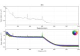
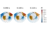

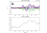
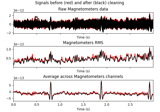
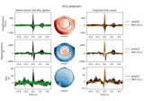
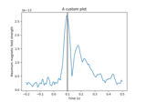
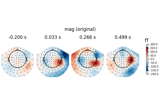
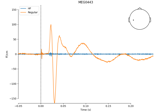
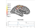
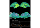
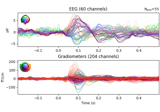
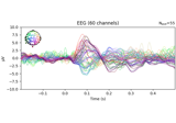
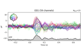
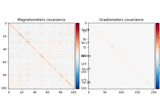
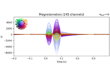
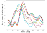
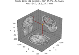
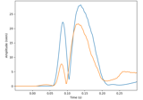

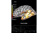

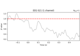
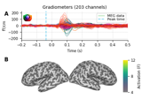
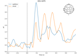
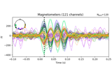
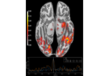
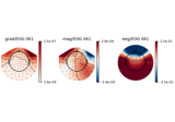
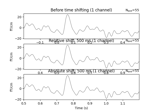
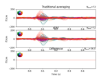

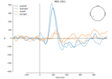
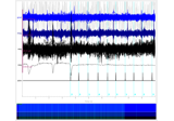
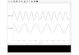
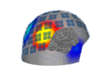
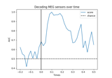
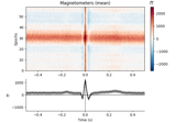
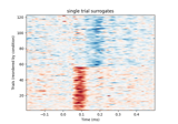
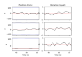
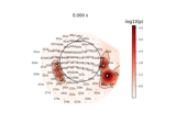
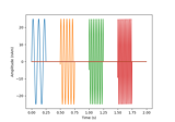
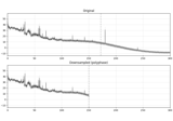
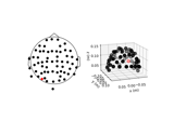
Examples using mne.Evoked#
Analysis of evoked response using ICA and PCA reduction techniques
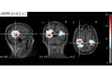
Compute MNE-dSPM inverse solution on evoked data in volume source space
Compute a sparse inverse solution using the Gamma-MAP empirical Bayesian method
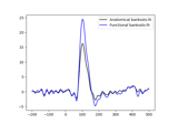
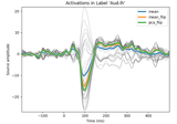
Extracting the time series of activations in a label
Compute sparse inverse solution with mixed norm: MxNE and irMxNE
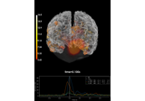
Compute MNE inverse solution on evoked data with a mixed source space
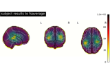
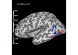
Plot point-spread functions (PSFs) and cross-talk functions (CTFs)

Compute spatial resolution metrics in source space
Compute spatial resolution metrics to compare MEG with EEG+MEG
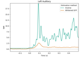
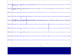
Plot sensor denoising using oversampled temporal projection
Analysing continuous features with binning and regression in sensor space
Compute source power spectral density (PSD) of VectorView and OPM data
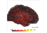
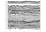
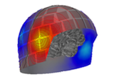
Source localization with equivalent current dipole (ECD) fit
The role of dipole orientations in distributed source localization
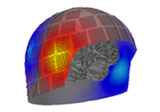
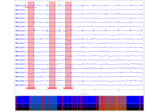
Visualising statistical significance thresholds on EEG data
Spatiotemporal permutation F-test on full sensor data
The Spectrum and EpochsSpectrum classes: frequency-domain data