Note
Click here to download the full example code
Compute source power spectral density (PSD) of VectorView and OPM data
Here we compute the resting state from raw for data recorded using a Neuromag VectorView system and a custom OPM system. The pipeline is meant to mostly follow the Brainstorm 1 OMEGA resting tutorial pipeline. The steps we use are:
Filtering: downsample heavily.
Artifact detection: use SSP for EOG and ECG.
Source localization: dSPM, depth weighting, cortically constrained.
Frequency: power spectral density (Welch), 4 sec window, 50% overlap.
Standardize: normalize by relative power for each source.
Preprocessing
# Authors: Denis Engemann <denis.engemann@gmail.com>
#          Luke Bloy <luke.bloy@gmail.com>
#          Eric Larson <larson.eric.d@gmail.com>
#
# License: BSD (3-clause)

import os.path as op

from mne.filter import next_fast_len

import mne


print(__doc__)

data_path = mne.datasets.opm.data_path()
subject = 'OPM_sample'

subjects_dir = op.join(data_path, 'subjects')
bem_dir = op.join(subjects_dir, subject, 'bem')
bem_fname = op.join(subjects_dir, subject, 'bem',
                    subject + '-5120-5120-5120-bem-sol.fif')
src_fname = op.join(bem_dir, '%s-oct6-src.fif' % subject)
vv_fname = data_path + '/MEG/SQUID/SQUID_resting_state.fif'
vv_erm_fname = data_path + '/MEG/SQUID/SQUID_empty_room.fif'
vv_trans_fname = data_path + '/MEG/SQUID/SQUID-trans.fif'
opm_fname = data_path + '/MEG/OPM/OPM_resting_state_raw.fif'
opm_erm_fname = data_path + '/MEG/OPM/OPM_empty_room_raw.fif'
opm_trans_fname = None
opm_coil_def_fname = op.join(data_path, 'MEG', 'OPM', 'coil_def.dat')
Load data, resample. We will store the raw objects in dicts with entries “vv” and “opm” to simplify housekeeping and simplify looping later.
raws = dict()
raw_erms = dict()
new_sfreq = 90.  # Nyquist frequency (45 Hz) < line noise freq (50 Hz)
raws['vv'] = mne.io.read_raw_fif(vv_fname, verbose='error')  # ignore naming
raws['vv'].load_data().resample(new_sfreq)
raws['vv'].info['bads'] = ['MEG2233', 'MEG1842']
raw_erms['vv'] = mne.io.read_raw_fif(vv_erm_fname, verbose='error')
raw_erms['vv'].load_data().resample(new_sfreq)
raw_erms['vv'].info['bads'] = ['MEG2233', 'MEG1842']

raws['opm'] = mne.io.read_raw_fif(opm_fname)
raws['opm'].load_data().resample(new_sfreq)
raw_erms['opm'] = mne.io.read_raw_fif(opm_erm_fname)
raw_erms['opm'].load_data().resample(new_sfreq)
# Make sure our assumptions later hold
assert raws['opm'].info['sfreq'] == raws['vv'].info['sfreq']
Out:
Opening raw data file /home/circleci/mne_data/MNE-OPM-data/MEG/OPM/OPM_resting_state_raw.fif...
Isotrak not found
    Range : 0 ... 61999 =      0.000 ...    61.999 secs
Ready.
Reading 0 ... 61999  =      0.000 ...    61.999 secs...
Trigger channel has a non-zero initial value of 256 (consider using initial_event=True to detect this event)
Trigger channel has a non-zero initial value of 256 (consider using initial_event=True to detect this event)
Opening raw data file /home/circleci/mne_data/MNE-OPM-data/MEG/OPM/OPM_empty_room_raw.fif...
Isotrak not found
    Range : 0 ... 61999 =      0.000 ...    61.999 secs
Ready.
Reading 0 ... 61999  =      0.000 ...    61.999 secs...
Trigger channel has a non-zero initial value of 256 (consider using initial_event=True to detect this event)
Trigger channel has a non-zero initial value of 256 (consider using initial_event=True to detect this event)
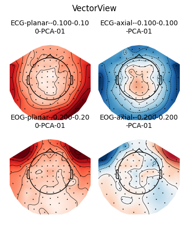
Do some minimal artifact rejection just for VectorView data
titles = dict(vv='VectorView', opm='OPM')
ssp_ecg, _ = mne.preprocessing.compute_proj_ecg(
    raws['vv'], tmin=-0.1, tmax=0.1, n_grad=1, n_mag=1)
raws['vv'].add_proj(ssp_ecg, remove_existing=True)
# due to how compute_proj_eog works, it keeps the old projectors, so
# the output contains both projector types (and also the original empty-room
# projectors)
ssp_ecg_eog, _ = mne.preprocessing.compute_proj_eog(
    raws['vv'], n_grad=1, n_mag=1, ch_name='MEG0112')
raws['vv'].add_proj(ssp_ecg_eog, remove_existing=True)
raw_erms['vv'].add_proj(ssp_ecg_eog)
fig = mne.viz.plot_projs_topomap(raws['vv'].info['projs'][-4:],
                                 info=raws['vv'].info)
fig.suptitle(titles['vv'])
fig.subplots_adjust(0.05, 0.05, 0.95, 0.85)
Out:
Including 13 SSP projectors from raw file
Running ECG SSP computation
Reconstructing ECG signal from Magnetometers
Setting up band-pass filter from 5 - 35 Hz

FIR filter parameters
---------------------
Designing a two-pass forward and reverse, zero-phase, non-causal bandpass filter:
- Windowed frequency-domain design (firwin2) method
- Hann window
- Lower passband edge: 5.00
- Lower transition bandwidth: 0.50 Hz (-12 dB cutoff frequency: 4.75 Hz)
- Upper passband edge: 35.00 Hz
- Upper transition bandwidth: 0.50 Hz (-12 dB cutoff frequency: 35.25 Hz)
- Filter length: 900 samples (10.000 sec)

Number of ECG events detected : 47 (average pulse 45 / min.)
Computing projector
Not setting metadata
Not setting metadata
47 matching events found
No baseline correction applied
Created an SSP operator (subspace dimension = 13)
13 projection items activated
Loading data for 47 events and 19 original time points ...
    Rejecting  epoch based on MAG : ['MEG0111']
1 bad epochs dropped
No EEG channels found. Forcing n_eeg to 0
Adding projection: planar--0.100-0.100-PCA-01
Adding projection: axial--0.100-0.100-PCA-01
Done.
Including 15 SSP projectors from raw file
Running EOG SSP computation
Using channel MEG0112 as EOG channel
EOG channel index for this subject is: [1]
Filtering the data to remove DC offset to help distinguish blinks from saccades
Setting up band-pass filter from 1 - 10 Hz

FIR filter parameters
---------------------
Designing a two-pass forward and reverse, zero-phase, non-causal bandpass filter:
- Windowed frequency-domain design (firwin2) method
- Hann window
- Lower passband edge: 1.00
- Lower transition bandwidth: 0.50 Hz (-12 dB cutoff frequency: 0.75 Hz)
- Upper passband edge: 10.00 Hz
- Upper transition bandwidth: 0.50 Hz (-12 dB cutoff frequency: 10.25 Hz)
- Filter length: 900 samples (10.000 sec)

Now detecting blinks and generating corresponding events
Found 40 significant peaks
Number of EOG events detected : 40
Computing projector
Not setting metadata
Not setting metadata
40 matching events found
No baseline correction applied
Created an SSP operator (subspace dimension = 15)
15 projection items activated
Loading data for 40 events and 37 original time points ...
    Rejecting  epoch based on MAG : ['MEG0111']
1 bad epochs dropped
No EEG channels found. Forcing n_eeg to 0
Adding projection: planar--0.200-0.200-PCA-01
Adding projection: axial--0.200-0.200-PCA-01
Done.
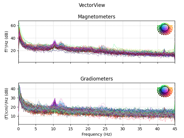
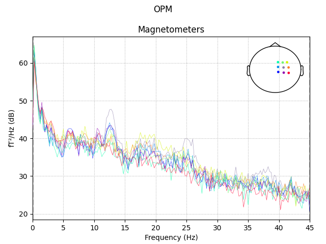
Explore data
Out:
Using n_fft=360 (4.0 sec)
No projector specified for this dataset. Please consider the method self.add_proj.
Effective window size : 4.000 (s)
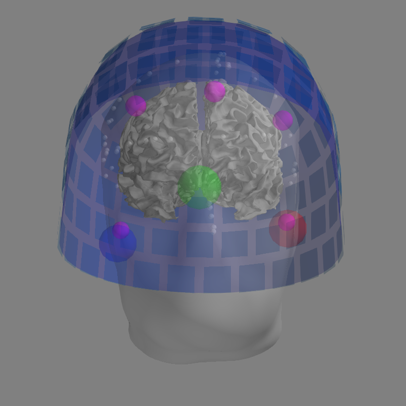
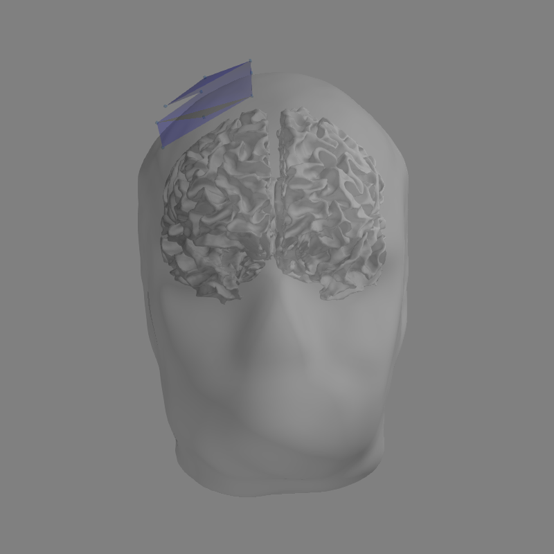
Alignment and forward
# Here we use a reduced size source space (oct5) just for speed
src = mne.setup_source_space(
    subject, 'oct5', add_dist=False, subjects_dir=subjects_dir)
# This line removes source-to-source distances that we will not need.
# We only do it here to save a bit of memory, in general this is not required.
del src[0]['dist'], src[1]['dist']
bem = mne.read_bem_solution(bem_fname)
fwd = dict()
trans = dict(vv=vv_trans_fname, opm=opm_trans_fname)
# check alignment and generate forward
with mne.use_coil_def(opm_coil_def_fname):
    for kind in kinds:
        dig = True if kind == 'vv' else False
        fig = mne.viz.plot_alignment(
            raws[kind].info, trans=trans[kind], subject=subject,
            subjects_dir=subjects_dir, dig=dig, coord_frame='mri',
            surfaces=('head', 'white'))
        mne.viz.set_3d_view(figure=fig, azimuth=0, elevation=90,
                            distance=0.6, focalpoint=(0., 0., 0.))
        fwd[kind] = mne.make_forward_solution(
            raws[kind].info, trans[kind], src, bem, eeg=False, verbose=True)
del trans, src, bem
Out:
Setting up the source space with the following parameters:

SUBJECTS_DIR = /home/circleci/mne_data/MNE-OPM-data/subjects
Subject      = OPM_sample
Surface      = white
Octahedron subdivision grade 5

>>> 1. Creating the source space...

Doing the octahedral vertex picking...
Loading /home/circleci/mne_data/MNE-OPM-data/subjects/OPM_sample/surf/lh.white...
Mapping lh OPM_sample -> oct (5) ...
    Triangle neighbors and vertex normals...
Loading geometry from /home/circleci/mne_data/MNE-OPM-data/subjects/OPM_sample/surf/lh.sphere...
Setting up the triangulation for the decimated surface...
loaded lh.white 1026/169022 selected to source space (oct = 5)

Loading /home/circleci/mne_data/MNE-OPM-data/subjects/OPM_sample/surf/rh.white...
Mapping rh OPM_sample -> oct (5) ...
    Triangle neighbors and vertex normals...
Loading geometry from /home/circleci/mne_data/MNE-OPM-data/subjects/OPM_sample/surf/rh.sphere...
Setting up the triangulation for the decimated surface...
loaded rh.white 1026/169992 selected to source space (oct = 5)

You are now one step closer to computing the gain matrix
Loading surfaces...

Loading the solution matrix...

Three-layer model surfaces loaded.
Loaded linear_collocation BEM solution from /home/circleci/mne_data/MNE-OPM-data/subjects/OPM_sample/bem/OPM_sample-5120-5120-5120-bem-sol.fif
Using outer_skin.surf for head surface.
Getting helmet for system 306m
Source space          : <SourceSpaces: [<surface (lh), n_vertices=169022, n_used=1026>, <surface (rh), n_vertices=169992, n_used=1026>] MRI (surface RAS) coords, subject 'OPM_sample', ~25.9 MB>
MRI -> head transform : /home/circleci/mne_data/MNE-OPM-data/MEG/SQUID/SQUID-trans.fif
Measurement data      : instance of Info
Conductor model   : instance of ConductorModel
Accurate field computations
Do computations in head coordinates
Free source orientations

Read 2 source spaces a total of 2052 active source locations

Coordinate transformation: MRI (surface RAS) -> head
     0.995623 -0.029776 -0.088592       1.15 mm
     0.062622  0.916188  0.395825       5.31 mm
     0.069381 -0.399641  0.914042      25.88 mm
     0.000000  0.000000  0.000000       1.00

Read 306 MEG channels from info
2 coil definitions read
99 coil definitions read
Coordinate transformation: MEG device -> head
     0.993107 -0.074371 -0.090590       0.76 mm
     0.079171  0.995577  0.050589     -13.97 mm
     0.086427 -0.057412  0.994603      60.91 mm
     0.000000  0.000000  0.000000       1.00
MEG coil definitions created in head coordinates.
Source spaces are now in head coordinates.

Employing the head->MRI coordinate transform with the BEM model.
BEM model instance of ConductorModel is now set up

Source spaces are in head coordinates.
Checking that the sources are inside the surface (will take a few...)
    Skipping interior check for 335 sources that fit inside a sphere of radius   51.5 mm
    Skipping solid angle check for 0 points using Qhull
    Skipping interior check for 334 sources that fit inside a sphere of radius   51.5 mm
    Skipping solid angle check for 0 points using Qhull

Setting up compensation data...
    No compensation set. Nothing more to do.

Composing the field computation matrix...
Computing MEG at 2052 source locations (free orientations)...

Finished.
Using outer_skin.surf for head surface.
Getting helmet for system unknown (derived from 9 MEG channel locations)
Source space          : <SourceSpaces: [<surface (lh), n_vertices=169022, n_used=1026>, <surface (rh), n_vertices=169992, n_used=1026>] MRI (surface RAS) coords, subject 'OPM_sample', ~25.9 MB>
MRI -> head transform : identity
Measurement data      : instance of Info
Conductor model   : instance of ConductorModel
Accurate field computations
Do computations in head coordinates
Free source orientations

Read 2 source spaces a total of 2052 active source locations

Coordinate transformation: MRI (surface RAS) -> head
     1.000000  0.000000  0.000000       0.00 mm
     0.000000  1.000000  0.000000       0.00 mm
     0.000000  0.000000  1.000000       0.00 mm
     0.000000  0.000000  0.000000       1.00

Read   9 MEG channels from info
2 coil definitions read
99 coil definitions read
Coordinate transformation: MEG device -> head
     0.999800  0.015800 -0.009200       0.10 mm
    -0.018100  0.930500 -0.365900      16.60 mm
     0.002800  0.366000  0.930600     -14.40 mm
     0.000000  0.000000  0.000000       1.00
MEG coil definitions created in head coordinates.
Source spaces are now in head coordinates.

Employing the head->MRI coordinate transform with the BEM model.
BEM model instance of ConductorModel is now set up

Source spaces are in head coordinates.
Checking that the sources are inside the surface (will take a few...)
    Skipping interior check for 335 sources that fit inside a sphere of radius   51.5 mm
    Skipping solid angle check for 0 points using Qhull
    Skipping interior check for 334 sources that fit inside a sphere of radius   51.5 mm
    Skipping solid angle check for 0 points using Qhull

Setting up compensation data...
    No compensation set. Nothing more to do.

Composing the field computation matrix...
Computing MEG at 2052 source locations (free orientations)...

Finished.
Compute and apply inverse to PSD estimated using multitaper + Welch. Group into frequency bands, then normalize each source point and sensor independently. This makes the value of each sensor point and source location in each frequency band the percentage of the PSD accounted for by that band.
freq_bands = dict(
    delta=(2, 4), theta=(5, 7), alpha=(8, 12), beta=(15, 29), gamma=(30, 45))
topos = dict(vv=dict(), opm=dict())
stcs = dict(vv=dict(), opm=dict())

snr = 3.
lambda2 = 1. / snr ** 2
for kind in kinds:
    noise_cov = mne.compute_raw_covariance(raw_erms[kind])
    inverse_operator = mne.minimum_norm.make_inverse_operator(
        raws[kind].info, forward=fwd[kind], noise_cov=noise_cov, verbose=True)
    stc_psd, sensor_psd = mne.minimum_norm.compute_source_psd(
        raws[kind], inverse_operator, lambda2=lambda2,
        n_fft=n_fft, dB=False, return_sensor=True, verbose=True)
    topo_norm = sensor_psd.data.sum(axis=1, keepdims=True)
    stc_norm = stc_psd.sum()  # same operation on MNE object, sum across freqs
    # Normalize each source point by the total power across freqs
    for band, limits in freq_bands.items():
        data = sensor_psd.copy().crop(*limits).data.sum(axis=1, keepdims=True)
        topos[kind][band] = mne.EvokedArray(
            100 * data / topo_norm, sensor_psd.info)
        stcs[kind][band] = \
            100 * stc_psd.copy().crop(*limits).sum() / stc_norm.data
    del inverse_operator
del fwd, raws, raw_erms
Out:
Using up to 305 segments
Number of samples used : 5490
[done]
Converting forward solution to surface orientation
    No patch info available. The standard source space normals will be employed in the rotation to the local surface coordinates....
    Converting to surface-based source orientations...
    [done]
info["bads"] and noise_cov["bads"] do not match, excluding bad channels from both
Computing inverse operator with 304 channels.
    304 out of 306 channels remain after picking
Selected 304 channels
Creating the depth weighting matrix...
    202 planar channels
    limit = 1968/2052 = 10.006596
    scale = 3.1863e-08 exp = 0.8
Applying loose dipole orientations to surface source spaces: 0.2
Whitening the forward solution.
    Created an SSP operator (subspace dimension = 17)
Computing rank from covariance with rank=None
    Using tolerance 7e-13 (2.2e-16 eps * 304 dim * 10  max singular value)
    Estimated rank (mag + grad): 287
    MEG: rank 287 computed from 304 data channels with 17 projectors
    Setting small MEG eigenvalues to zero (without PCA)
Creating the source covariance matrix
Adjusting source covariance matrix.
Computing SVD of whitened and weighted lead field matrix.
    largest singular value = 6.41665
    scaling factor to adjust the trace = 3.36215e+19
Not setting metadata
Not setting metadata
31 matching events found
No baseline correction applied
Created an SSP operator (subspace dimension = 17)
17 projection items activated
Considering frequencies 0 ... 200 Hz
Preparing the inverse operator for use...
    Scaled noise and source covariance from nave = 1 to nave = 1
    Created the regularized inverter
    Created an SSP operator (subspace dimension = 17)
    Created the whitener using a noise covariance matrix with rank 287 (17 small eigenvalues omitted)
    Computing noise-normalization factors (dSPM)...
[done]
Picked 304 channels from the data
Computing inverse...
    Eigenleads need to be weighted ...
Reducing data rank 304 -> 287
Using hann windowing on at most 31 epochs

  0%|          |  : 0/31 [00:00<?,       ?it/s]
  3%|3         |  : 1/31 [00:00<00:02,   13.67it/s]
  6%|6         |  : 2/31 [00:00<00:02,   13.74it/s]
 10%|9         |  : 3/31 [00:00<00:02,   13.81it/s]
 13%|#2        |  : 4/31 [00:00<00:01,   13.93it/s]
 16%|#6        |  : 5/31 [00:00<00:01,   14.05it/s]
 19%|#9        |  : 6/31 [00:00<00:01,   14.14it/s]
 23%|##2       |  : 7/31 [00:00<00:01,   14.24it/s]
 26%|##5       |  : 8/31 [00:00<00:01,   14.31it/s]
 29%|##9       |  : 9/31 [00:00<00:01,   14.40it/s]
 32%|###2      |  : 10/31 [00:00<00:01,   14.51it/s]
 35%|###5      |  : 11/31 [00:00<00:01,   14.59it/s]
 39%|###8      |  : 12/31 [00:00<00:01,   14.67it/s]
 42%|####1     |  : 13/31 [00:00<00:01,   14.74it/s]
 45%|####5     |  : 14/31 [00:00<00:01,   14.79it/s]
 48%|####8     |  : 15/31 [00:00<00:01,   14.89it/s]
 52%|#####1    |  : 16/31 [00:00<00:01,   14.99it/s]
 55%|#####4    |  : 17/31 [00:01<00:00,   15.08it/s]
 58%|#####8    |  : 18/31 [00:01<00:00,   15.16it/s]
 61%|######1   |  : 19/31 [00:01<00:00,   15.25it/s]
 65%|######4   |  : 20/31 [00:01<00:00,   15.33it/s]
 68%|######7   |  : 21/31 [00:01<00:00,   15.40it/s]
 71%|#######   |  : 22/31 [00:01<00:00,   15.47it/s]
 74%|#######4  |  : 23/31 [00:01<00:00,   15.45it/s]
 77%|#######7  |  : 24/31 [00:01<00:00,   15.52it/s]
 81%|########  |  : 25/31 [00:01<00:00,   15.55it/s]
 84%|########3 |  : 26/31 [00:01<00:00,   15.59it/s]
 87%|########7 |  : 27/31 [00:01<00:00,   15.59it/s]
 90%|######### |  : 28/31 [00:01<00:00,   15.58it/s]
 94%|#########3|  : 29/31 [00:01<00:00,   15.57it/s]
 97%|#########6|  : 30/31 [00:01<00:00,   15.52it/s]
 97%|#########6|  : 30/31 [00:01<00:00,   16.11it/s]
Using up to 310 segments
Number of samples used : 5580
[done]
Converting forward solution to surface orientation
    No patch info available. The standard source space normals will be employed in the rotation to the local surface coordinates....
    Converting to surface-based source orientations...
    [done]
Computing inverse operator with 9 channels.
    9 out of 9 channels remain after picking
Selected 9 channels
Creating the depth weighting matrix...
    9 magnetometer or axial gradiometer channels
    limit = 1696/2052 = 10.002109
    scale = 5.16226e-11 exp = 0.8
Applying loose dipole orientations to surface source spaces: 0.2
Whitening the forward solution.
Computing rank from covariance with rank=None
    Using tolerance 3e-13 (2.2e-16 eps * 9 dim * 1.5e+02  max singular value)
    Estimated rank (mag): 9
    MAG: rank 9 computed from 9 data channels with 0 projectors
    Setting small MAG eigenvalues to zero (without PCA)
Creating the source covariance matrix
Adjusting source covariance matrix.
Computing SVD of whitened and weighted lead field matrix.
    largest singular value = 2.44062
    scaling factor to adjust the trace = 4.31379e+17
Not setting metadata
Not setting metadata
31 matching events found
No baseline correction applied
0 projection items activated
Considering frequencies 0 ... 200 Hz
Preparing the inverse operator for use...
    Scaled noise and source covariance from nave = 1 to nave = 1
    Created the regularized inverter
    The projection vectors do not apply to these channels.
    Created the whitener using a noise covariance matrix with rank 9 (0 small eigenvalues omitted)
    Computing noise-normalization factors (dSPM)...
[done]
Picked 9 channels from the data
Computing inverse...
    Eigenleads need to be weighted ...
Reducing data rank 9 -> 9
Using hann windowing on at most 31 epochs

  0%|          |  : 0/31 [00:00<?,       ?it/s]
  3%|3         |  : 1/31 [00:00<00:01,   27.65it/s]
  6%|6         |  : 2/31 [00:00<00:01,   27.39it/s]
 10%|9         |  : 3/31 [00:00<00:01,   27.30it/s]
 13%|#2        |  : 4/31 [00:00<00:00,   27.39it/s]
 16%|#6        |  : 5/31 [00:00<00:00,   27.46it/s]
 19%|#9        |  : 6/31 [00:00<00:00,   27.58it/s]
 23%|##2       |  : 7/31 [00:00<00:00,   27.67it/s]
 26%|##5       |  : 8/31 [00:00<00:00,   27.74it/s]
 29%|##9       |  : 9/31 [00:00<00:00,   27.84it/s]
 32%|###2      |  : 10/31 [00:00<00:00,   27.90it/s]
 35%|###5      |  : 11/31 [00:00<00:00,   27.97it/s]
 39%|###8      |  : 12/31 [00:00<00:00,   28.06it/s]
 42%|####1     |  : 13/31 [00:00<00:00,   28.11it/s]
 45%|####5     |  : 14/31 [00:00<00:00,   28.22it/s]
 48%|####8     |  : 15/31 [00:00<00:00,   28.33it/s]
 52%|#####1    |  : 16/31 [00:00<00:00,   28.35it/s]
 55%|#####4    |  : 17/31 [00:00<00:00,   28.34it/s]
 58%|#####8    |  : 18/31 [00:00<00:00,   28.29it/s]
 61%|######1   |  : 19/31 [00:00<00:00,   28.32it/s]
 65%|######4   |  : 20/31 [00:00<00:00,   28.27it/s]
 68%|######7   |  : 21/31 [00:00<00:00,   28.31it/s]
 71%|#######   |  : 22/31 [00:00<00:00,   28.39it/s]
 74%|#######4  |  : 23/31 [00:00<00:00,   28.41it/s]
 77%|#######7  |  : 24/31 [00:00<00:00,   28.43it/s]
 81%|########  |  : 25/31 [00:00<00:00,   28.45it/s]
 84%|########3 |  : 26/31 [00:00<00:00,   28.47it/s]
 87%|########7 |  : 27/31 [00:00<00:00,   28.51it/s]
 90%|######### |  : 28/31 [00:00<00:00,   28.52it/s]
 94%|#########3|  : 29/31 [00:01<00:00,   28.57it/s]
 97%|#########6|  : 30/31 [00:01<00:00,   28.57it/s]
 97%|#########6|  : 30/31 [00:01<00:00,   28.66it/s]
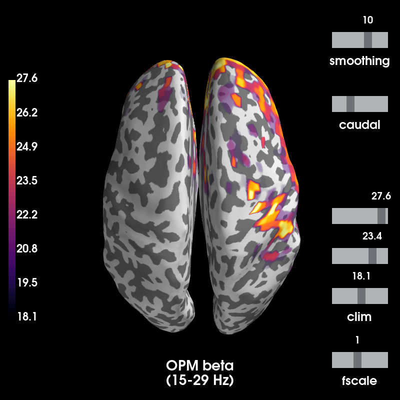
Now we can make some plots of each frequency band. Note that the OPM head coverage is only over right motor cortex, so only localization of beta is likely to be worthwhile.
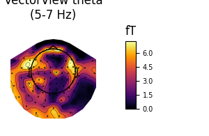
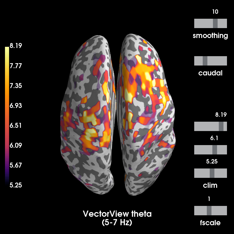
Theta
def plot_band(kind, band):
    """Plot activity within a frequency band on the subject's brain."""
    title = "%s %s\n(%d-%d Hz)" % ((titles[kind], band,) + freq_bands[band])
    topos[kind][band].plot_topomap(
        times=0., scalings=1., cbar_fmt='%0.1f', vmin=0, cmap='inferno',
        time_format=title)
    brain = stcs[kind][band].plot(
        subject=subject, subjects_dir=subjects_dir, views='cau', hemi='both',
        time_label=title, title=title, colormap='inferno',
        clim=dict(kind='percent', lims=(70, 85, 99)), smoothing_steps=10)
    brain.show_view(dict(azimuth=0, elevation=0), roll=0)
    return fig, brain


fig_theta, brain_theta = plot_band('vv', 'theta')
Out:
Removing projector <Projection | ECG-planar--0.100-0.100-PCA-01, active : True, n_channels : 202>
Removing projector <Projection | EOG-planar--0.200-0.200-PCA-01, active : True, n_channels : 202>
Using control points [5.25322167 6.10014818 8.19402478]
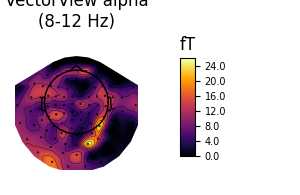
Alpha
fig_alpha, brain_alpha = plot_band('vv', 'alpha')
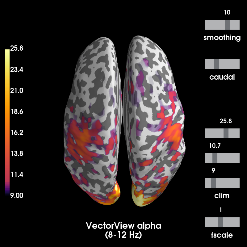
Out:
Removing projector <Projection | ECG-planar--0.100-0.100-PCA-01, active : True, n_channels : 202>
Removing projector <Projection | EOG-planar--0.200-0.200-PCA-01, active : True, n_channels : 202>
Using control points [ 8.9970254  10.71727163 25.82171392]
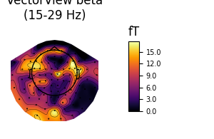
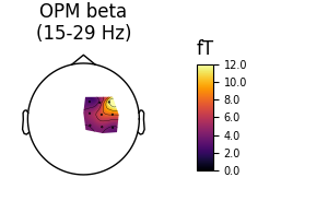
Beta
Here we also show OPM data, which shows a profile similar to the VectorView data beneath the sensors.
fig_beta, brain_beta = plot_band('vv', 'beta')
fig_beta_opm, brain_beta_opm = plot_band('opm', 'beta')
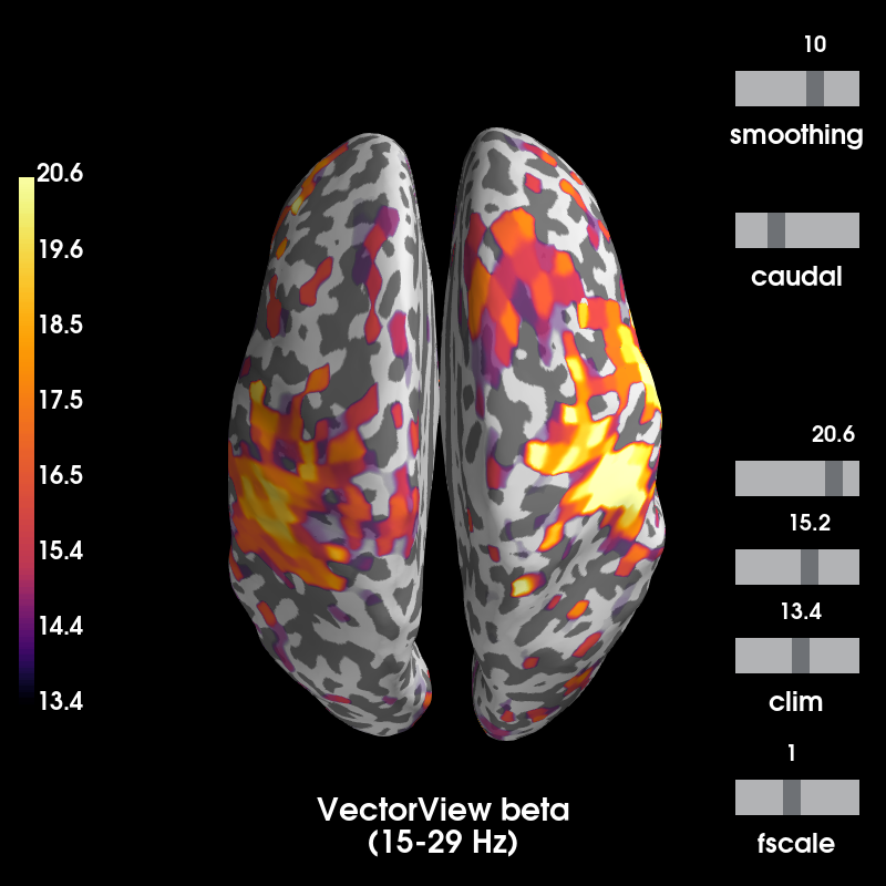
Out:
Removing projector <Projection | ECG-planar--0.100-0.100-PCA-01, active : True, n_channels : 202>
Removing projector <Projection | EOG-planar--0.200-0.200-PCA-01, active : True, n_channels : 202>
Using control points [13.35796725 15.23048388 20.58456084]
Using control points [18.11773229 23.40740491 27.55664771]
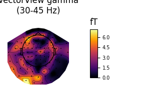
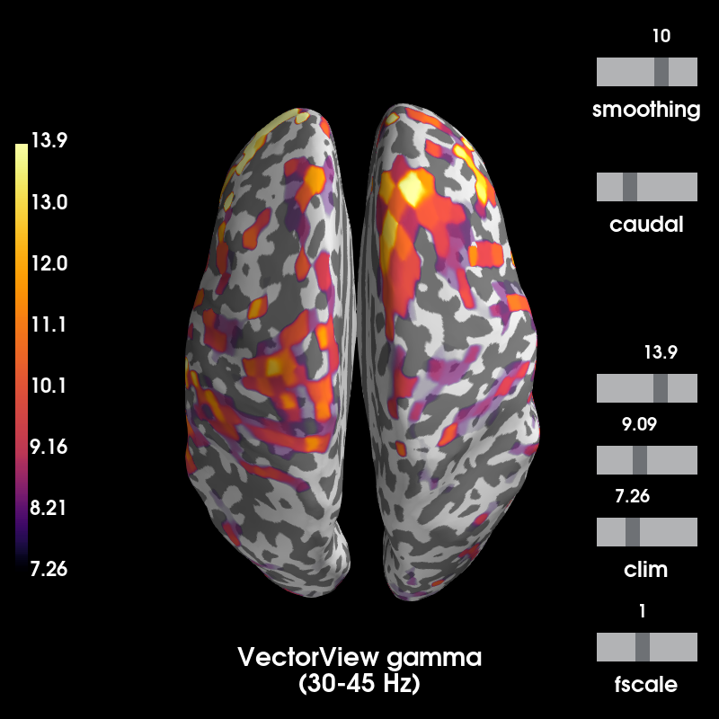
Gamma
fig_gamma, brain_gamma = plot_band('vv', 'gamma')
Out:
Removing projector <Projection | ECG-planar--0.100-0.100-PCA-01, active : True, n_channels : 202>
Removing projector <Projection | EOG-planar--0.200-0.200-PCA-01, active : True, n_channels : 202>
Using control points [ 7.26102199  9.09179916 13.91323047]
References
- 1
Tadel F, Baillet S, Mosher JC, Pantazis D, Leahy RM. Brainstorm: A User-Friendly Application for MEG/EEG Analysis. Computational Intelligence and Neuroscience, vol. 2011, Article ID 879716, 13 pages, 2011. doi:10.1155/2011/879716
Total running time of the script: ( 1 minutes 17.339 seconds)
Estimated memory usage: 619 MB