Note
Click here to download the full example code
DICS for power mapping
In this tutorial, we’ll simulate two signals originating from two locations on the cortex. These signals will be sinusoids, so we’ll be looking at oscillatory activity (as opposed to evoked activity).
We’ll use dynamic imaging of coherent sources (DICS) 1 to map out spectral power along the cortex. Let’s see if we can find our two simulated sources.
# Author: Marijn van Vliet <w.m.vanvliet@gmail.com>
#
# License: BSD (3-clause)
Setup
We first import the required packages to run this tutorial and define a list of filenames for various things we’ll be using.
import os.path as op
import numpy as np
from scipy.signal import welch, coherence, unit_impulse
from matplotlib import pyplot as plt

import mne
from mne.simulation import simulate_raw, add_noise
from mne.datasets import sample
from mne.minimum_norm import make_inverse_operator, apply_inverse
from mne.time_frequency import csd_morlet
from mne.beamformer import make_dics, apply_dics_csd

# We use the MEG and MRI setup from the MNE-sample dataset
data_path = sample.data_path(download=False)
subjects_dir = op.join(data_path, 'subjects')

# Filenames for various files we'll be using
meg_path = op.join(data_path, 'MEG', 'sample')
raw_fname = op.join(meg_path, 'sample_audvis_raw.fif')
fwd_fname = op.join(meg_path, 'sample_audvis-meg-eeg-oct-6-fwd.fif')
cov_fname = op.join(meg_path, 'sample_audvis-cov.fif')
fwd = mne.read_forward_solution(fwd_fname)

# Seed for the random number generator
rand = np.random.RandomState(42)
Out:
Reading forward solution from /home/circleci/mne_data/MNE-sample-data/MEG/sample/sample_audvis-meg-eeg-oct-6-fwd.fif...
    Reading a source space...
    Computing patch statistics...
    Patch information added...
    Distance information added...
    [done]
    Reading a source space...
    Computing patch statistics...
    Patch information added...
    Distance information added...
    [done]
    2 source spaces read
    Desired named matrix (kind = 3523) not available
    Read MEG forward solution (7498 sources, 306 channels, free orientations)
    Desired named matrix (kind = 3523) not available
    Read EEG forward solution (7498 sources, 60 channels, free orientations)
    MEG and EEG forward solutions combined
    Source spaces transformed to the forward solution coordinate frame
Data simulation
The following function generates a timeseries that contains an oscillator, whose frequency fluctuates a little over time, but stays close to 10 Hz. We’ll use this function to generate our two signals.
sfreq = 50.  # Sampling frequency of the generated signal
n_samp = int(round(10. * sfreq))
times = np.arange(n_samp) / sfreq  # 10 seconds of signal
n_times = len(times)


def coh_signal_gen():
    """Generate an oscillating signal.

    Returns
    -------
    signal : ndarray
        The generated signal.
    """
    t_rand = 0.001  # Variation in the instantaneous frequency of the signal
    std = 0.1  # Std-dev of the random fluctuations added to the signal
    base_freq = 10.  # Base frequency of the oscillators in Hertz
    n_times = len(times)

    # Generate an oscillator with varying frequency and phase lag.
    signal = np.sin(2.0 * np.pi *
                    (base_freq * np.arange(n_times) / sfreq +
                     np.cumsum(t_rand * rand.randn(n_times))))

    # Add some random fluctuations to the signal.
    signal += std * rand.randn(n_times)

    # Scale the signal to be in the right order of magnitude (~100 nAm)
    # for MEG data.
    signal *= 100e-9

    return signal
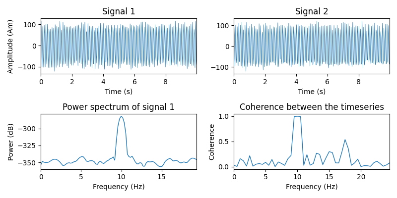
Let’s simulate two timeseries and plot some basic information about them.
signal1 = coh_signal_gen()
signal2 = coh_signal_gen()

fig, axes = plt.subplots(2, 2, figsize=(8, 4))

# Plot the timeseries
ax = axes[0][0]
ax.plot(times, 1e9 * signal1, lw=0.5)
ax.set(xlabel='Time (s)', xlim=times[[0, -1]], ylabel='Amplitude (Am)',
       title='Signal 1')
ax = axes[0][1]
ax.plot(times, 1e9 * signal2, lw=0.5)
ax.set(xlabel='Time (s)', xlim=times[[0, -1]], title='Signal 2')

# Power spectrum of the first timeseries
f, p = welch(signal1, fs=sfreq, nperseg=128, nfft=256)
ax = axes[1][0]
# Only plot the first 100 frequencies
ax.plot(f[:100], 20 * np.log10(p[:100]), lw=1.)
ax.set(xlabel='Frequency (Hz)', xlim=f[[0, 99]],
       ylabel='Power (dB)', title='Power spectrum of signal 1')

# Compute the coherence between the two timeseries
f, coh = coherence(signal1, signal2, fs=sfreq, nperseg=100, noverlap=64)
ax = axes[1][1]
ax.plot(f[:50], coh[:50], lw=1.)
ax.set(xlabel='Frequency (Hz)', xlim=f[[0, 49]], ylabel='Coherence',
       title='Coherence between the timeseries')
fig.tight_layout()
Now we put the signals at two locations on the cortex. We construct a
mne.SourceEstimate object to store them in.
The timeseries will have a part where the signal is active and a part where it is not. The techniques we’ll be using in this tutorial depend on being able to contrast data that contains the signal of interest versus data that does not (i.e. it contains only noise).
# The locations on the cortex where the signal will originate from. These
# locations are indicated as vertex numbers.
vertices = [[146374], [33830]]

# Construct SourceEstimates that describe the signals at the cortical level.
data = np.vstack((signal1, signal2))
stc_signal = mne.SourceEstimate(
    data, vertices, tmin=0, tstep=1. / sfreq, subject='sample')
stc_noise = stc_signal * 0.
Before we simulate the sensor-level data, let’s define a signal-to-noise ratio. You are encouraged to play with this parameter and see the effect of noise on our results.
snr = 1. # Signal-to-noise ratio. Decrease to add more noise.
Now we run the signal through the forward model to obtain simulated sensor data. To save computation time, we’ll only simulate gradiometer data. You can try simulating other types of sensors as well.
Some noise is added based on the baseline noise covariance matrix from the sample dataset, scaled to implement the desired SNR.
# Read the info from the sample dataset. This defines the location of the
# sensors and such.
info = mne.io.read_info(raw_fname)
info.update(sfreq=sfreq, bads=[])

# Only use gradiometers
picks = mne.pick_types(info, meg='grad', stim=True, exclude=())
mne.pick_info(info, picks, copy=False)

# Define a covariance matrix for the simulated noise. In this tutorial, we use
# a simple diagonal matrix.
cov = mne.cov.make_ad_hoc_cov(info)
cov['data'] *= (20. / snr) ** 2  # Scale the noise to achieve the desired SNR

# Simulate the raw data, with a lowpass filter on the noise
stcs = [(stc_signal, unit_impulse(n_samp, dtype=int) * 1),
        (stc_noise, unit_impulse(n_samp, dtype=int) * 2)]  # stacked in time
duration = (len(stc_signal.times) * 2) / sfreq
raw = simulate_raw(info, stcs, forward=fwd)
add_noise(raw, cov, iir_filter=[4, -4, 0.8], random_state=rand)
Out:
    Read a total of 3 projection items:
        PCA-v1 (1 x 10²)  idle
        PCA-v2 (1 x 10²)  idle
        PCA-v3 (1 x 10²)  idle
Setting up raw simulation: 1 position, "cos2" interpolation
Event information stored on channel:              STI 014
    Interval 0.000-10.000 sec
Setting up forward solutions
Computing gain matrix for transform #1/1
    Interval 0.000-10.000 sec
    2 STC iterations provided
Done
Adding noise to 204/213 channels (204 channels in cov)
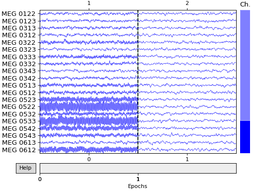
We create an mne.Epochs object containing two trials: one with
both noise and signal and one with just noise
events = mne.find_events(raw, initial_event=True)
tmax = (len(stc_signal.times) - 1) / sfreq
epochs = mne.Epochs(raw, events, event_id=dict(signal=1, noise=2),
                    tmin=0, tmax=tmax, baseline=None, preload=True)
assert len(epochs) == 2  # ensure that we got the two expected events

# Plot some of the channels of the simulated data that are situated above one
# of our simulated sources.
picks = mne.pick_channels(epochs.ch_names, mne.read_selection('Left-frontal'))
epochs.plot(picks=picks)
Out:
2 events found
Event IDs: [1 2]
Not setting metadata
Not setting metadata
2 matching events found
No baseline correction applied
3 projection items activated
Loading data for 2 events and 500 original time points ...
0 bad epochs dropped
Power mapping
With our simulated dataset ready, we can now pretend to be researchers that have just recorded this from a real subject and are going to study what parts of the brain communicate with each other.
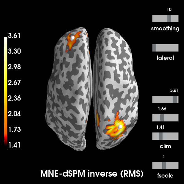
First, we’ll create a source estimate of the MEG data. We’ll use both a straightforward MNE-dSPM inverse solution for this, and the DICS beamformer which is specifically designed to work with oscillatory data.
Computing the inverse using MNE-dSPM:
# Compute the inverse operator
fwd = mne.read_forward_solution(fwd_fname)
inv = make_inverse_operator(epochs.info, fwd, cov)

# Apply the inverse model to the trial that also contains the signal.
s = apply_inverse(epochs['signal'].average(), inv)

# Take the root-mean square along the time dimension and plot the result.
s_rms = np.sqrt((s ** 2).mean())
title = 'MNE-dSPM inverse (RMS)'
brain = s_rms.plot('sample', subjects_dir=subjects_dir, hemi='both', figure=1,
                   size=600, time_label=title, title=title)

# Indicate the true locations of the source activity on the plot.
brain.add_foci(vertices[0][0], coords_as_verts=True, hemi='lh')
brain.add_foci(vertices[1][0], coords_as_verts=True, hemi='rh')

# Rotate the view and add a title.
brain.show_view(view={'azimuth': 0, 'elevation': 0, 'distance': 550,
                'focalpoint': [0, 0, 0]})
Out:
Reading forward solution from /home/circleci/mne_data/MNE-sample-data/MEG/sample/sample_audvis-meg-eeg-oct-6-fwd.fif...
    Reading a source space...
    Computing patch statistics...
    Patch information added...
    Distance information added...
    [done]
    Reading a source space...
    Computing patch statistics...
    Patch information added...
    Distance information added...
    [done]
    2 source spaces read
    Desired named matrix (kind = 3523) not available
    Read MEG forward solution (7498 sources, 306 channels, free orientations)
    Desired named matrix (kind = 3523) not available
    Read EEG forward solution (7498 sources, 60 channels, free orientations)
    MEG and EEG forward solutions combined
    Source spaces transformed to the forward solution coordinate frame
Converting forward solution to surface orientation
    Average patch normals will be employed in the rotation to the local surface coordinates....
    Converting to surface-based source orientations...
    [done]
Computing inverse operator with 204 channels.
    204 out of 366 channels remain after picking
Selected 204 channels
Creating the depth weighting matrix...
    204 planar channels
    limit = 7261/7498 = 10.004929
    scale = 2.59947e-08 exp = 0.8
Applying loose dipole orientations to surface source spaces: 0.2
Whitening the forward solution.
Computing rank from covariance with rank=None
    Using tolerance 4.5e-14 (2.2e-16 eps * 204 dim * 1  max singular value)
    Estimated rank (grad): 204
    GRAD: rank 204 computed from 204 data channels with 0 projectors
    Setting small GRAD eigenvalues to zero (without PCA)
Creating the source covariance matrix
Adjusting source covariance matrix.
Computing SVD of whitened and weighted lead field matrix.
    largest singular value = 5.60587
    scaling factor to adjust the trace = 2.91651e+18
Removing projector <Projection | PCA-v1, active : True, n_channels : 102>
Removing projector <Projection | PCA-v2, active : True, n_channels : 102>
Removing projector <Projection | PCA-v3, active : True, n_channels : 102>
Preparing the inverse operator for use...
    Scaled noise and source covariance from nave = 1 to nave = 1
    Created the regularized inverter
    The projection vectors do not apply to these channels.
    Created the whitener using a noise covariance matrix with rank 204 (0 small eigenvalues omitted)
    Computing noise-normalization factors (dSPM)...
[done]
Applying inverse operator to "signal"...
    Picked 204 channels from the data
    Computing inverse...
    Eigenleads need to be weighted ...
    Computing residual...
    Explained  75.0% variance
    Combining the current components...
    dSPM...
[done]
Using control points [1.41101364 1.65792783 3.61406449]
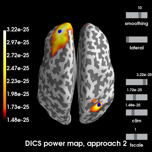
We will now compute the cortical power map at 10 Hz. using a DICS beamformer. A beamformer will construct for each vertex a spatial filter that aims to pass activity originating from the vertex, while dampening activity from other sources as much as possible.
The mne.beamformer.make_dics() function has many switches that offer
precise control
over the way the filter weights are computed. Currently, there is no clear
consensus regarding the best approach. This is why we will demonstrate two
approaches here:
# Estimate the cross-spectral density (CSD) matrix on the trial containing the
# signal.
csd_signal = csd_morlet(epochs['signal'], frequencies=[10])
# Compute the spatial filters for each vertex, using two approaches.
filters_approach1 = make_dics(
info, fwd, csd_signal, reg=0.05, pick_ori='max-power', depth=1.,
inversion='single', weight_norm=None)
print(filters_approach1)
filters_approach2 = make_dics(
info, fwd, csd_signal, reg=0.05, pick_ori='max-power', depth=None,
inversion='matrix', weight_norm='unit-noise-gain')
print(filters_approach2)
# You can save these to disk with:
# filters_approach1.save('filters_1-dics.h5')
# Compute the DICS power map by applying the spatial filters to the CSD matrix.
power_approach1, f = apply_dics_csd(csd_signal, filters_approach1)
power_approach2, f = apply_dics_csd(csd_signal, filters_approach2)
# Plot the DICS power maps for both approaches.
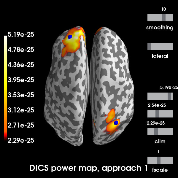
brains = list()
for approach, power in enumerate([power_approach1, power_approach2], 1):
title = 'DICS power map, approach %d' % approach
brain = power.plot('sample', subjects_dir=subjects_dir, hemi='both',
figure=approach + 1, size=600, time_label=title,
title=title)
# Indicate the true locations of the source activity on the plot.
brain.add_foci(vertices[0][0], coords_as_verts=True, hemi='lh', color='b')
brain.add_foci(vertices[1][0], coords_as_verts=True, hemi='rh', color='b')
# Rotate the view and add a title.
brain.show_view(view={'azimuth': 0, 'elevation': 0, 'distance': 550,
'focalpoint': [0, 0, 0]})
brains.append(brain)
Out:
Removing projector <Projection | PCA-v1, active : True, n_channels : 102>
Removing projector <Projection | PCA-v2, active : True, n_channels : 102>
Removing projector <Projection | PCA-v3, active : True, n_channels : 102>
Computing cross-spectral density from epochs...
    Computing CSD matrix for epoch 1
[done]
Identifying common channels ...
Dropped the following channels:
['EEG 027', 'MEG 1211', 'MEG 0531', 'MEG 0911', 'MEG 0931', 'EEG 017', 'MEG 2041', 'MEG 1921', 'MEG 2231', 'EEG 024', 'MEG 1511', 'EEG 047', 'EEG 054', 'EEG 060', 'STI 002', 'STI 014', 'MEG 1721', 'MEG 1731', 'MEG 0121', 'MEG 1121', 'MEG 0411', 'MEG 2141', 'MEG 0241', 'MEG 2631', 'EEG 002', 'EEG 008', 'EEG 031', 'MEG 2311', 'MEG 0131', 'MEG 1831', 'MEG 1421', 'EEG 023', 'MEG 1431', 'EEG 011', 'MEG 2421', 'EEG 045', 'EEG 049', 'MEG 1241', 'EEG 022', 'EEG 030', 'MEG 0711', 'MEG 2441', 'MEG 1941', 'MEG 0441', 'STI 003', 'MEG 1541', 'EEG 040', 'MEG 0321', 'MEG 0541', 'MEG 2331', 'MEG 0211', 'MEG 2541', 'MEG 1841', 'MEG 0511', 'MEG 1821', 'EEG 056', 'EEG 007', 'EEG 001', 'MEG 1641', 'EEG 048', 'EEG 003', 'MEG 2221', 'EEG 006', 'MEG 1411', 'MEG 0631', 'MEG 0141', 'EEG 039', 'MEG 2131', 'EEG 034', 'EEG 032', 'MEG 1141', 'EEG 055', 'EEG 051', 'EEG 053', 'MEG 1911', 'STI 005', 'MEG 1021', 'MEG 1031', 'EEG 052', 'MEG 0111', 'EEG 038', 'EEG 035', 'EEG 019', 'STI 004', 'MEG 1331', 'MEG 2031', 'MEG 2411', 'MEG 1231', 'MEG 2621', 'MEG 1441', 'MEG 1041', 'MEG 0621', 'EEG 004', 'MEG 1631', 'MEG 1131', 'MEG 2121', 'MEG 0641', 'EEG 009', 'MEG 2021', 'EEG 036', 'EEG 046', 'MEG 2641', 'EEG 033', 'EEG 044', 'MEG 1111', 'EEG 058', 'MEG 1221', 'MEG 1531', 'MEG 2011', 'EEG 059', 'EEG 016', 'MEG 0821', 'MEG 1611', 'MEG 1931', 'EEG 050', 'MEG 2431', 'MEG 0611', 'MEG 0941', 'MEG 2321', 'MEG 1741', 'MEG 0421', 'MEG 2211', 'MEG 2531', 'MEG 1711', 'MEG 2611', 'EEG 013', 'MEG 0331', 'MEG 0431', 'EEG 043', 'MEG 1811', 'MEG 0221', 'MEG 2341', 'MEG 0741', 'MEG 0341', 'EEG 005', 'MEG 1621', 'EEG 042', 'MEG 0521', 'EEG 020', 'MEG 0921', 'STI 015', 'STI 006', 'EEG 029', 'EEG 037', 'EEG 018', 'MEG 1341', 'MEG 2521', 'MEG 0731', 'EEG 026', 'MEG 1521', 'MEG 2511', 'EEG 028', 'EEG 015', 'EEG 010', 'MEG 1011', 'MEG 0721', 'EEG 041', 'EEG 012', 'STI 016', 'MEG 1321', 'MEG 0811', 'MEG 1311', 'STI 001', 'EEG 057', 'MEG 0231', 'MEG 0311', 'EEG 021', 'EEG 014', 'MEG 2111', 'MEG 2241', 'EEG 025']
Computing inverse operator with 204 channels.
    204 out of 366 channels remain after picking
Selected 204 channels
Creating the depth weighting matrix...
Whitening the forward solution.
Computing rank from covariance with rank=None
    Using tolerance 4.5e+08 (2.2e-16 eps * 204 dim * 1e+22  max singular value)
    Estimated rank (grad): 204
    GRAD: rank 204 computed from 204 data channels with 0 projectors
    Setting small GRAD eigenvalues to zero (without PCA)
Creating the source covariance matrix
Adjusting source covariance matrix.
Computing DICS spatial filters...
Computing beamformer filters for 7498 sources
Filter computation complete
<Beamformer | DICS, subject "sample", 7498 vert, 204 ch, max-power ori, single inversion>
Identifying common channels ...
Dropped the following channels:
['EEG 027', 'MEG 1211', 'MEG 0531', 'MEG 0911', 'MEG 0931', 'EEG 017', 'MEG 2041', 'MEG 1921', 'MEG 2231', 'EEG 024', 'MEG 1511', 'EEG 047', 'EEG 054', 'EEG 060', 'STI 002', 'STI 014', 'MEG 1721', 'MEG 1731', 'MEG 0121', 'MEG 1121', 'MEG 0411', 'MEG 2141', 'MEG 0241', 'MEG 2631', 'EEG 002', 'EEG 008', 'EEG 031', 'MEG 2311', 'MEG 0131', 'MEG 1831', 'MEG 1421', 'EEG 023', 'MEG 1431', 'EEG 011', 'MEG 2421', 'EEG 045', 'EEG 049', 'MEG 1241', 'EEG 022', 'EEG 030', 'MEG 0711', 'MEG 2441', 'MEG 1941', 'MEG 0441', 'STI 003', 'MEG 1541', 'EEG 040', 'MEG 0321', 'MEG 0541', 'MEG 2331', 'MEG 0211', 'MEG 2541', 'MEG 1841', 'MEG 0511', 'MEG 1821', 'EEG 056', 'EEG 007', 'EEG 001', 'MEG 1641', 'EEG 048', 'EEG 003', 'MEG 2221', 'EEG 006', 'MEG 1411', 'MEG 0631', 'MEG 0141', 'EEG 039', 'MEG 2131', 'EEG 034', 'EEG 032', 'MEG 1141', 'EEG 055', 'EEG 051', 'EEG 053', 'MEG 1911', 'STI 005', 'MEG 1021', 'MEG 1031', 'EEG 052', 'MEG 0111', 'EEG 038', 'EEG 035', 'EEG 019', 'STI 004', 'MEG 1331', 'MEG 2031', 'MEG 2411', 'MEG 1231', 'MEG 2621', 'MEG 1441', 'MEG 1041', 'MEG 0621', 'EEG 004', 'MEG 1631', 'MEG 1131', 'MEG 2121', 'MEG 0641', 'EEG 009', 'MEG 2021', 'EEG 036', 'EEG 046', 'MEG 2641', 'EEG 033', 'EEG 044', 'MEG 1111', 'EEG 058', 'MEG 1221', 'MEG 1531', 'MEG 2011', 'EEG 059', 'EEG 016', 'MEG 0821', 'MEG 1611', 'MEG 1931', 'EEG 050', 'MEG 2431', 'MEG 0611', 'MEG 0941', 'MEG 2321', 'MEG 1741', 'MEG 0421', 'MEG 2211', 'MEG 2531', 'MEG 1711', 'MEG 2611', 'EEG 013', 'MEG 0331', 'MEG 0431', 'EEG 043', 'MEG 1811', 'MEG 0221', 'MEG 2341', 'MEG 0741', 'MEG 0341', 'EEG 005', 'MEG 1621', 'EEG 042', 'MEG 0521', 'EEG 020', 'MEG 0921', 'STI 015', 'STI 006', 'EEG 029', 'EEG 037', 'EEG 018', 'MEG 1341', 'MEG 2521', 'MEG 0731', 'EEG 026', 'MEG 1521', 'MEG 2511', 'EEG 028', 'EEG 015', 'EEG 010', 'MEG 1011', 'MEG 0721', 'EEG 041', 'EEG 012', 'STI 016', 'MEG 1321', 'MEG 0811', 'MEG 1311', 'STI 001', 'EEG 057', 'MEG 0231', 'MEG 0311', 'EEG 021', 'EEG 014', 'MEG 2111', 'MEG 2241', 'EEG 025']
Computing inverse operator with 204 channels.
    204 out of 366 channels remain after picking
Selected 204 channels
Whitening the forward solution.
Computing rank from covariance with rank=None
    Using tolerance 4.5e+08 (2.2e-16 eps * 204 dim * 1e+22  max singular value)
    Estimated rank (grad): 204
    GRAD: rank 204 computed from 204 data channels with 0 projectors
    Setting small GRAD eigenvalues to zero (without PCA)
Creating the source covariance matrix
Adjusting source covariance matrix.
Computing DICS spatial filters...
Computing beamformer filters for 7498 sources
Filter computation complete
<Beamformer | DICS, subject "sample", 7498 vert, 204 ch, max-power ori, unit-noise-gain norm, matrix inversion>
Computing DICS source power...
[done]
Computing DICS source power...
[done]
Using control points [2.29171434e-25 2.53680419e-25 5.18967629e-25]
Using control points [1.48256606e-25 1.71721566e-25 3.21604646e-25]
Excellent! All methods found our two simulated sources. Of course, with a signal-to-noise ratio (SNR) of 1, is isn’t very hard to find them. You can try playing with the SNR and see how the MNE-dSPM and DICS approaches hold up in the presence of increasing noise. In the presence of more noise, you may need to increase the regularization parameter of the DICS beamformer.
References
- 1
Gross et al. (2001). Dynamic imaging of coherent sources: Studying neural interactions in the human brain. Proceedings of the National Academy of Sciences, 98(2), 694-699. https://doi.org/10.1073/pnas.98.2.694
- 2
van Vliet, et al. (2018) Analysis of functional connectivity and oscillatory power using DICS: from raw MEG data to group-level statistics in Python. bioRxiv, 245530. https://doi.org/10.1101/245530
- 3
Sekihara & Nagarajan. Adaptive spatial filters for electromagnetic brain imaging (2008) Springer Science & Business Media
Total running time of the script: ( 0 minutes 29.487 seconds)
Estimated memory usage: 290 MB