Source alignment and coordinate frames

This tutorial shows how to visually assess the spatial alignment of MEG sensor locations, digitized scalp landmark and sensor locations, and MRI volumes. This alignment process is crucial for computing the forward solution, as is understanding the different coordinate frames involved in this process.

Let’s start out by loading some data.

import os.path as op

import numpy as np
import nibabel as nib
from scipy import linalg

import mne
from mne.io.constants import FIFF

data_path = mne.datasets.sample.data_path()
subjects_dir = op.join(data_path, 'subjects')
raw_fname = op.join(data_path, 'MEG', 'sample', 'sample_audvis_raw.fif')
trans_fname = op.join(data_path, 'MEG', 'sample',
                      'sample_audvis_raw-trans.fif')
raw = mne.io.read_raw_fif(raw_fname)
trans = mne.read_trans(trans_fname)
src = mne.read_source_spaces(op.join(subjects_dir, 'sample', 'bem',
                                     'sample-oct-6-src.fif'))

# load the T1 file and change the header information to the correct units
t1w = nib.load(op.join(data_path, 'subjects', 'sample', 'mri', 'T1.mgz'))
t1w = nib.Nifti1Image(t1w.dataobj, t1w.affine)
t1w.header['xyzt_units'] = np.array(10, dtype='uint8')
t1_mgh = nib.MGHImage(t1w.dataobj, t1w.affine)

Out:

Opening raw data file /home/circleci/mne_data/MNE-sample-data/MEG/sample/sample_audvis_raw.fif...
    Read a total of 3 projection items:
        PCA-v1 (1 x 102)  idle
        PCA-v2 (1 x 102)  idle
        PCA-v3 (1 x 102)  idle
    Range : 25800 ... 192599 =     42.956 ...   320.670 secs
Ready.
    Reading a source space...
    Computing patch statistics...
    Patch information added...
    Distance information added...
    [done]
    Reading a source space...
    Computing patch statistics...
    Patch information added...
    Distance information added...
    [done]
    2 source spaces read

Understanding coordinate frames

For M/EEG source imaging, there are three coordinate frames must be brought into alignment using two 3D transformation matrices that define how to rotate and translate points in one coordinate frame to their equivalent locations in another. The three main coordinate frames are:

• “meg”: the coordinate frame for the physical locations of MEG sensors

• “mri”: the coordinate frame for MRI images, and scalp/skull/brain surfaces derived from the MRI images

• “head”: the coordinate frame for digitized sensor locations and scalp landmarks (“fiducials”)

Each of these are described in more detail in the next section.

A good way to start visualizing these coordinate frames is to use the mne.viz.plot_alignment function, which is used for creating or inspecting the transformations that bring these coordinate frames into alignment, and displaying the resulting alignment of EEG sensors, MEG sensors, brain sources, and conductor models. If you provide subjects_dir and subject parameters, the function automatically loads the subject’s Freesurfer MRI surfaces. Important for our purposes, passing show_axes=True to plot_alignment will draw the origin of each coordinate frame in a different color, with axes indicated by different sized arrows:

• shortest arrow: (R)ight / X

• medium arrow: forward / (A)nterior / Y

• longest arrow: up / (S)uperior / Z

Note that all three coordinate systems are RAS coordinate frames and hence are also right-handed coordinate systems. Finally, note that the coord_frame parameter sets which coordinate frame the camera should initially be aligned with. Let’s take a look:

fig = mne.viz.plot_alignment(raw.info, trans=trans, subject='sample',
                             subjects_dir=subjects_dir, surfaces='head-dense',
                             show_axes=True, dig=True, eeg=[], meg='sensors',
                             coord_frame='meg')
mne.viz.set_3d_view(fig, 45, 90, distance=0.6, focalpoint=(0., 0., 0.))
print('Distance from head origin to MEG origin: %0.1f mm'
      % (1000 * np.linalg.norm(raw.info['dev_head_t']['trans'][:3, 3])))
print('Distance from head origin to MRI origin: %0.1f mm'
      % (1000 * np.linalg.norm(trans['trans'][:3, 3])))
dists = mne.dig_mri_distances(raw.info, trans, 'sample',
                              subjects_dir=subjects_dir)
print('Distance from %s digitized points to head surface: %0.1f mm'
      % (len(dists), 1000 * np.mean(dists)))

Out:

Using lh.seghead for head surface.
Distance from head origin to MEG origin: 65.0 mm
Distance from head origin to MRI origin: 29.9 mm
Using surface from /home/circleci/mne_data/MNE-sample-data/subjects/sample/bem/sample-head.fif.
Distance from 72 digitized points to head surface: 1.7 mm

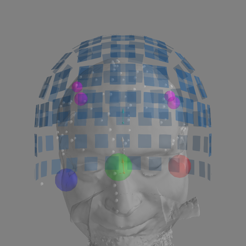
Coordinate frame definitions

1. Neuromag/Elekta/MEGIN head coordinate frame (“head”, pink axes)

   The head coordinate frame is defined through the coordinates of anatomical landmarks on the subject’s head: usually the Nasion (NAS), and the left and right preauricular points (LPA and RPA). Different MEG manufacturers may have different definitions of the head coordinate frame. A good overview can be seen in the FieldTrip FAQ on coordinate systems.

   For Neuromag/Elekta/MEGIN, the head coordinate frame is defined by the intersection of

   1. the line between the LPA (red sphere) and RPA (purple sphere), and

   2. the line perpendicular to this LPA-RPA line one that goes through the Nasion (green sphere).

   The axes are oriented as X origin→RPA, Y origin→NAS, Z origin→upward (orthogonal to X and Y).

   Note

   The required 3D coordinates for defining the head coordinate frame (NAS, LPA, RPA) are measured at a stage separate from the MEG data recording. There exist numerous devices to perform such measurements, usually called “digitizers”. For example, see the devices by the company Polhemus.

2. MEG device coordinate frame (“meg”, blue axes)

   The MEG device coordinate frame is defined by the respective MEG manufacturers. All MEG data is acquired with respect to this coordinate frame. To account for the anatomy and position of the subject’s head, we use so-called head position indicator (HPI) coils. The HPI coils are placed at known locations on the scalp of the subject and emit high-frequency magnetic fields used to coregister the head coordinate frame with the device coordinate frame.

   From the Neuromag/Elekta/MEGIN user manual:

   The origin of the device coordinate system is located at the center of the posterior spherical section of the helmet with X axis going from left to right and Y axis pointing front. The Z axis is, again normal to the plane with positive direction up.

   Note

   The HPI coils are shown as magenta spheres. Coregistration happens at the beginning of the recording and the head↔meg transformation matrix is stored in raw.info['dev_head_t'].

3. MRI coordinate frame (“mri”, gray axes)

   Defined by Freesurfer, the “MRI surface RAS” coordinate frame has its origin at the center of a 256×256×256 1mm anisotropic volume (though the center may not correspond to the anatomical center of the subject’s head).

   Note

   We typically align the MRI coordinate frame to the head coordinate frame through a rotation and translation matrix, that we refer to in MNE as trans.

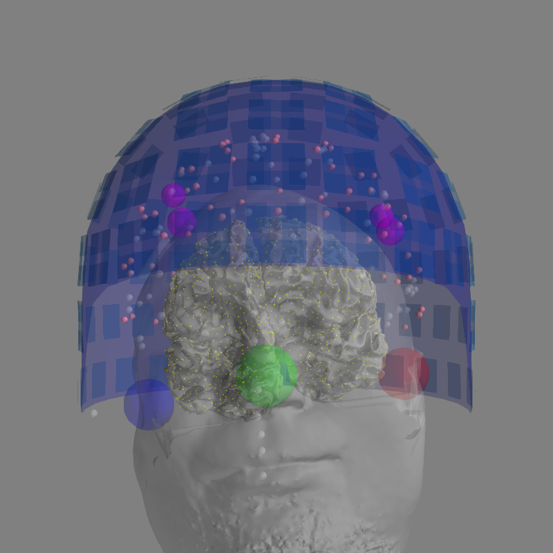
A bad example

Let’s try using plot_alignment with trans=None, which (incorrectly!) equates the MRI and head coordinate frames.

mne.viz.plot_alignment(raw.info, trans=None, subject='sample', src=src,
                       subjects_dir=subjects_dir, dig=True,
                       surfaces=['head-dense', 'white'], coord_frame='meg')

Out:

Using lh.seghead for head surface.
Getting helmet for system 306m

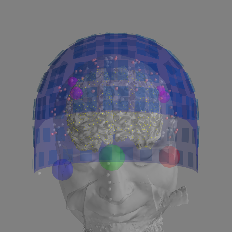
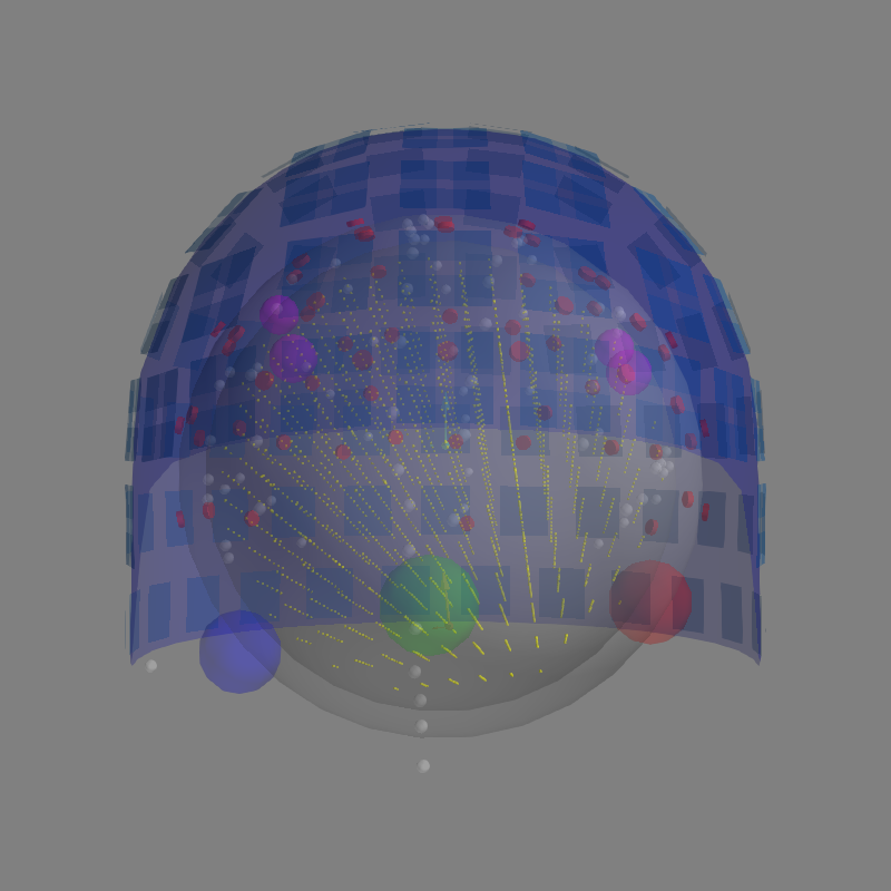
A good example

Here is the same plot, this time with the trans properly defined (using a precomputed transformation matrix).

mne.viz.plot_alignment(raw.info, trans=trans, subject='sample',
                       src=src, subjects_dir=subjects_dir, dig=True,
                       surfaces=['head-dense', 'white'], coord_frame='meg')

Out:

Using lh.seghead for head surface.
Getting helmet for system 306m

Visualizing the transformations

Let’s visualize these coordinate frames using just the scalp surface; this will make it easier to see their relative orientations. To do this we’ll first load the Freesurfer scalp surface, then apply a few different transforms to it. In addition to the three coordinate frames discussed above, we’ll also show the “mri_voxel” coordinate frame. Unlike MRI Surface RAS, “mri_voxel” has its origin in the corner of the volume (the left-most, posterior-most coordinate on the inferior-most MRI slice) instead of at the center of the volume. “mri_voxel” is also not an RAS coordinate system: rather, its XYZ directions are based on the acquisition order of the T1 image slices.

# the head surface is stored in "mri" coordinate frame
# (origin at center of volume, units=mm)
seghead_rr, seghead_tri = mne.read_surface(
    op.join(subjects_dir, 'sample', 'surf', 'lh.seghead'))

# to put the scalp in the "head" coordinate frame, we apply the inverse of
# the precomputed `trans` (which maps head → mri)
mri_to_head = linalg.inv(trans['trans'])
scalp_pts_in_head_coord = mne.transforms.apply_trans(
    mri_to_head, seghead_rr, move=True)

# to put the scalp in the "meg" coordinate frame, we use the inverse of
# raw.info['dev_head_t']
head_to_meg = linalg.inv(raw.info['dev_head_t']['trans'])
scalp_pts_in_meg_coord = mne.transforms.apply_trans(
    head_to_meg, scalp_pts_in_head_coord, move=True)

# The "mri_voxel"→"mri" transform is embedded in the header of the T1 image
# file. We'll invert it and then apply it to the original `seghead_rr` points.
# No unit conversion necessary: this transform expects mm and the scalp surface
# is defined in mm.
vox_to_mri = t1_mgh.header.get_vox2ras_tkr()
mri_to_vox = linalg.inv(vox_to_mri)
scalp_points_in_vox = mne.transforms.apply_trans(
    mri_to_vox, seghead_rr, move=True)

Now that we’ve transformed all the points, let’s plot them. We’ll use the same colors used by plot_alignment and use green for the “mri_voxel” coordinate frame:

def add_head(renderer, points, color, opacity=0.95):
    renderer.mesh(*points.T, triangles=seghead_tri, color=color,
                  opacity=opacity)


renderer = mne.viz.backends.renderer.create_3d_figure(
    size=(600, 600), bgcolor='w', scene=False)
add_head(renderer, seghead_rr, 'gray')
add_head(renderer, scalp_pts_in_meg_coord, 'blue')
add_head(renderer, scalp_pts_in_head_coord, 'pink')
add_head(renderer, scalp_points_in_vox, 'green')
mne.viz.set_3d_view(figure=renderer.figure, distance=800,
                    focalpoint=(0., 30., 30.), elevation=105, azimuth=180)
renderer.show()

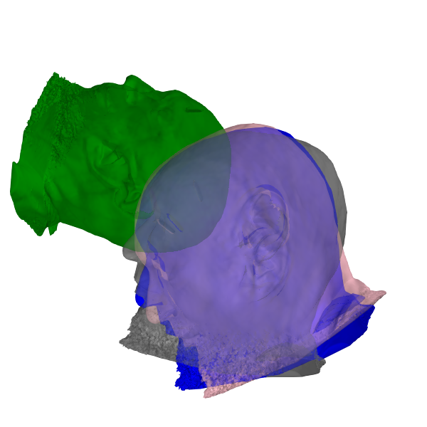
The relative orientations of the coordinate frames can be inferred by observing the direction of the subject’s nose. Notice also how the origin of the mri_voxel coordinate frame is in the corner of the volume (above, behind, and to the left of the subject), whereas the other three coordinate frames have their origin roughly in the center of the head.

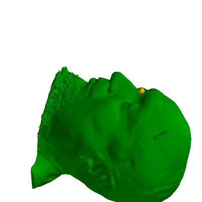
Example: MRI defacing

For a real-world example of using these transforms, consider the task of defacing the MRI to preserve subject anonymity. If you know the points in the “head” coordinate frame (as you might if you’re basing the defacing on digitized points) you would need to transform them into “mri” or “mri_voxel” in order to apply the blurring or smoothing operations to the MRI surfaces or images. Here’s what that would look like (we’ll use the nasion landmark as a representative example):

# get the nasion
nasion = [p for p in raw.info['dig'] if
          p['kind'] == FIFF.FIFFV_POINT_CARDINAL and
          p['ident'] == FIFF.FIFFV_POINT_NASION][0]
assert nasion['coord_frame'] == FIFF.FIFFV_COORD_HEAD
nasion = nasion['r']  # get just the XYZ values

# transform it from head to MRI space (recall that `trans` is head → mri)
nasion_mri = mne.transforms.apply_trans(trans, nasion, move=True)
# then transform to voxel space, after converting from meters to millimeters
nasion_vox = mne.transforms.apply_trans(
    mri_to_vox, nasion_mri * 1e3, move=True)
# plot it to make sure the transforms worked
renderer = mne.viz.backends.renderer.create_3d_figure(
    size=(400, 400), bgcolor='w', scene=False)
add_head(renderer, scalp_points_in_vox, 'green', opacity=1)
renderer.sphere(center=nasion_vox, color='orange', scale=10)
mne.viz.set_3d_view(figure=renderer.figure, distance=600.,
                    focalpoint=(0., 125., 250.), elevation=45, azimuth=180)
renderer.show()

Defining the head↔MRI trans using the GUI

You can try creating the head↔MRI transform yourself using mne.gui.coregistration().

• First you must load the digitization data from the raw file (Head Shape Source). The MRI data is already loaded if you provide the subject and subjects_dir. Toggle Always Show Head Points to see the digitization points.

• To set the landmarks, toggle Edit radio button in MRI Fiducials.

• Set the landmarks by clicking the radio button (LPA, Nasion, RPA) and then clicking the corresponding point in the image.

• After doing this for all the landmarks, toggle Lock radio button. You can omit outlier points, so that they don’t interfere with the finetuning.

  Note

  You can save the fiducials to a file and pass mri_fiducials=True to plot them in mne.viz.plot_alignment(). The fiducials are saved to the subject’s bem folder by default.

• Click Fit Head Shape. This will align the digitization points to the head surface. Sometimes the fitting algorithm doesn’t find the correct alignment immediately. You can try first fitting using LPA/RPA or fiducials and then align according to the digitization. You can also finetune manually with the controls on the right side of the panel.

• Click Save As... (lower right corner of the panel), set the filename and read it with mne.read_trans().

For more information, see step by step instructions in these slides. Uncomment the following line to align the data yourself.

# mne.gui.coregistration(subject='sample', subjects_dir=subjects_dir)

Alignment without MRI

The surface alignments above are possible if you have the surfaces available from Freesurfer. mne.viz.plot_alignment() automatically searches for the correct surfaces from the provided subjects_dir. Another option is to use a spherical conductor model. It is passed through bem parameter.

sphere = mne.make_sphere_model(info=raw.info, r0='auto', head_radius='auto')
src = mne.setup_volume_source_space(sphere=sphere, pos=10.)
mne.viz.plot_alignment(
    raw.info, eeg='projected', bem=sphere, src=src, dig=True,
    surfaces=['brain', 'outer_skin'], coord_frame='meg', show_axes=True)

Out:

Fitted sphere radius:         91.0 mm
Origin head coordinates:      -4.1 16.0 51.7 mm
Origin device coordinates:    1.4 17.8 -10.3 mm

Equiv. model fitting -> RV = 0.00349028 %
mu1 = 0.944696    lambda1 = 0.137193
mu2 = 0.667458    lambda2 = 0.683737
mu3 = -0.26815    lambda3 = -0.0105603
Set up EEG sphere model with scalp radius    91.0 mm

Sphere                : origin at (-4.1 16.0 51.7) mm
              radius  : 81.9 mm
grid                  : 10.0 mm
mindist               : 5.0 mm

Setting up the sphere...
Surface CM = (  -4.1   16.0   51.7) mm
Surface fits inside a sphere with radius   81.9 mm
Surface extent:
    x =  -86.0 ...   77.8 mm
    y =  -65.9 ...   97.9 mm
    z =  -30.2 ...  133.7 mm
Grid extent:
    x =  -90.0 ...   80.0 mm
    y =  -70.0 ...  100.0 mm
    z =  -40.0 ...  140.0 mm
6156 sources before omitting any.
2300 sources after omitting infeasible sources not within 0.0 - 81.9 mm.
1904 sources remaining after excluding the sources outside the surface and less than    5.0 mm inside.
Adjusting the neighborhood info.
Source space : MRI voxel -> MRI (surface RAS)
     0.010000  0.000000  0.000000     -90.00 mm
     0.000000  0.010000  0.000000     -70.00 mm
     0.000000  0.000000  0.010000     -40.00 mm
     0.000000  0.000000  0.000000       1.00
Getting helmet for system 306m
    Triangle neighbors and vertex normals...

It is also possible to use mne.gui.coregistration() to warp a subject (usually fsaverage) to subject digitization data, see these slides.

Estimated memory usage: 23 MB