Note
Click here to download the full example code
Compute envelope correlations in source space
Compute envelope correlations of orthogonalized activity 12 in source space using resting state CTF data.
# Authors: Eric Larson <larson.eric.d@gmail.com>
#          Sheraz Khan <sheraz@khansheraz.com>
#          Denis Engemann <denis.engemann@gmail.com>
#
# License: BSD (3-clause)

import os.path as op

import numpy as np
import matplotlib.pyplot as plt

import mne
from mne.connectivity import envelope_correlation
from mne.minimum_norm import make_inverse_operator, apply_inverse_epochs
from mne.preprocessing import compute_proj_ecg, compute_proj_eog

data_path = mne.datasets.brainstorm.bst_resting.data_path()
subjects_dir = op.join(data_path, 'subjects')
subject = 'bst_resting'
trans = op.join(data_path, 'MEG', 'bst_resting', 'bst_resting-trans.fif')
src = op.join(subjects_dir, subject, 'bem', subject + '-oct-6-src.fif')
bem = op.join(subjects_dir, subject, 'bem', subject + '-5120-bem-sol.fif')
raw_fname = op.join(data_path, 'MEG', 'bst_resting',
                    'subj002_spontaneous_20111102_01_AUX.ds')
Here we do some things in the name of speed, such as crop (which will hurt SNR) and downsample. Then we compute SSP projectors and apply them.
raw = mne.io.read_raw_ctf(raw_fname, verbose='error')
raw.crop(0, 60).pick_types(meg=True, eeg=False).load_data().resample(80)
raw.apply_gradient_compensation(3)
projs_ecg, _ = compute_proj_ecg(raw, n_grad=1, n_mag=2)
projs_eog, _ = compute_proj_eog(raw, n_grad=1, n_mag=2, ch_name='MLT31-4407')
raw.info['projs'] += projs_ecg
raw.info['projs'] += projs_eog
raw.apply_proj()
cov = mne.compute_raw_covariance(raw)  # compute before band-pass of interest
Out:
Including 0 SSP projectors from raw file
Running ECG SSP computation
Reconstructing ECG signal from Magnetometers
Setting up band-pass filter from 5 - 35 Hz

FIR filter parameters
---------------------
Designing a two-pass forward and reverse, zero-phase, non-causal bandpass filter:
- Windowed frequency-domain design (firwin2) method
- Hann window
- Lower passband edge: 5.00
- Lower transition bandwidth: 0.50 Hz (-12 dB cutoff frequency: 4.75 Hz)
- Upper passband edge: 35.00 Hz
- Upper transition bandwidth: 0.50 Hz (-12 dB cutoff frequency: 35.25 Hz)
- Filter length: 800 samples (10.000 sec)

Number of ECG events detected : 88 (average pulse 88 / min.)
Computing projector
Not setting metadata
Not setting metadata
88 matching events found
No baseline correction applied
0 projection items activated
Loading data for 88 events and 49 original time points ...
    Rejecting  epoch based on MAG : ['MLT31-4407', 'MRT31-4407']
    Rejecting  epoch based on MAG : ['MLT31-4407', 'MLT41-4407', 'MRT31-4407', 'MRT41-4407']
    Rejecting  epoch based on MAG : ['MLT31-4407', 'MLT41-4407', 'MRT31-4407', 'MRT41-4407']
4 bad epochs dropped
No gradiometers found. Forcing n_grad to 0
No EEG channels found. Forcing n_eeg to 0
Adding projection: axial--0.200-0.400-PCA-01
Adding projection: axial--0.200-0.400-PCA-02
Done.
Including 0 SSP projectors from raw file
Running EOG SSP computation
Using channel MLT31-4407 as EOG channel
EOG channel index for this subject is: [137]
Filtering the data to remove DC offset to help distinguish blinks from saccades
Setting up band-pass filter from 1 - 10 Hz

FIR filter parameters
---------------------
Designing a two-pass forward and reverse, zero-phase, non-causal bandpass filter:
- Windowed frequency-domain design (firwin2) method
- Hann window
- Lower passband edge: 1.00
- Lower transition bandwidth: 0.50 Hz (-12 dB cutoff frequency: 0.75 Hz)
- Upper passband edge: 10.00 Hz
- Upper transition bandwidth: 0.50 Hz (-12 dB cutoff frequency: 10.25 Hz)
- Filter length: 800 samples (10.000 sec)

Now detecting blinks and generating corresponding events
Found 12 significant peaks
Number of EOG events detected : 12
Computing projector
Not setting metadata
Not setting metadata
12 matching events found
No baseline correction applied
0 projection items activated
Loading data for 12 events and 33 original time points ...
    Rejecting  epoch based on MAG : ['MRT41-4407']
1 bad epochs dropped
No gradiometers found. Forcing n_grad to 0
No EEG channels found. Forcing n_eeg to 0
Adding projection: axial--0.200-0.200-PCA-01
Adding projection: axial--0.200-0.200-PCA-02
Done.
Using up to 300 segments
Number of samples used : 4800
[done]
Now we band-pass filter our data and create epochs.
raw.filter(14, 30)
events = mne.make_fixed_length_events(raw, duration=5.)
epochs = mne.Epochs(raw, events=events, tmin=0, tmax=5.,
                    baseline=None, reject=dict(mag=8e-13), preload=True)
del raw
Out:
Not setting metadata
Not setting metadata
12 matching events found
No baseline correction applied
Created an SSP operator (subspace dimension = 4)
4 projection items activated
Loading data for 12 events and 401 original time points ...
    Rejecting  epoch based on MAG : ['MRC42-4407', 'MRC54-4407', 'MRP12-4407', 'MRP22-4407', 'MRP23-4407']
2 bad epochs dropped
Compute the forward and inverse
src = mne.read_source_spaces(src)
fwd = mne.make_forward_solution(epochs.info, trans, src, bem)
inv = make_inverse_operator(epochs.info, fwd, cov)
del fwd, src
Out:
    Reading a source space...
    Computing patch statistics...
    Patch information added...
    Distance information added...
    [done]
    Reading a source space...
    Computing patch statistics...
    Patch information added...
    Distance information added...
    [done]
    2 source spaces read
Source space          : <SourceSpaces: [<surface (lh), n_vertices=156869, n_used=4098>, <surface (rh), n_vertices=155654, n_used=4098>] MRI (surface RAS) coords, subject 'bst_resting', ~27.4 MB>
MRI -> head transform : /home/circleci/mne_data/MNE-brainstorm-data/bst_resting/MEG/bst_resting/bst_resting-trans.fif
Measurement data      : instance of Info
Conductor model   : /home/circleci/mne_data/MNE-brainstorm-data/bst_resting/subjects/bst_resting/bem/bst_resting-5120-bem-sol.fif
Accurate field computations
Do computations in head coordinates
Free source orientations

Read 2 source spaces a total of 8196 active source locations

Coordinate transformation: MRI (surface RAS) -> head
     0.999797 -0.005775 -0.019288       2.71 mm
     0.011390  0.952195  0.305279      16.66 mm
     0.016602 -0.305437  0.952068      28.47 mm
     0.000000  0.000000  0.000000       1.00

Read 272 MEG channels from info
Read  26 MEG compensation channels from info
99 coil definitions read
Coordinate transformation: MEG device -> head
     0.998490 -0.050225 -0.022235       1.90 mm
     0.052235  0.993447  0.101656      13.13 mm
     0.016984 -0.102664  0.994571      66.69 mm
     0.000000  0.000000  0.000000       1.00
5 compensation data sets in info
MEG coil definitions created in head coordinates.
Removing 5 compensators from info because not all compensation channels were picked.
Source spaces are now in head coordinates.

Setting up the BEM model using /home/circleci/mne_data/MNE-brainstorm-data/bst_resting/subjects/bst_resting/bem/bst_resting-5120-bem-sol.fif...

Loading surfaces...

Loading the solution matrix...

Homogeneous model surface loaded.
Loaded linear_collocation BEM solution from /home/circleci/mne_data/MNE-brainstorm-data/bst_resting/subjects/bst_resting/bem/bst_resting-5120-bem-sol.fif
Employing the head->MRI coordinate transform with the BEM model.
BEM model bst_resting-5120-bem-sol.fif is now set up

Source spaces are in head coordinates.
Checking that the sources are inside the surface (will take a few...)
    Skipping interior check for 1239 sources that fit inside a sphere of radius   49.6 mm
    Skipping solid angle check for 0 points using Qhull
    Skipping interior check for 1235 sources that fit inside a sphere of radius   49.6 mm
    Skipping solid angle check for 0 points using Qhull

Setting up compensation data...
    272 out of 272 channels have the compensation set.
    Desired compensation data (3) found.
    All compensation channels found.
    Preselector created.
    Compensation data matrix created.
    Postselector created.

Composing the field computation matrix...
Composing the field computation matrix (compensation coils)...
Computing MEG at 8196 source locations (free orientations)...

Finished.
Converting forward solution to surface orientation
    Average patch normals will be employed in the rotation to the local surface coordinates....
    Converting to surface-based source orientations...
    [done]
Computing inverse operator with 272 channels.
    272 out of 272 channels remain after picking
Removing 5 compensators from info because not all compensation channels were picked.
Selected 272 channels
Creating the depth weighting matrix...
    272 magnetometer or axial gradiometer channels
    limit = 8074/8196 = 10.006553
    scale = 5.92189e-11 exp = 0.8
Applying loose dipole orientations to surface source spaces: 0.2
Whitening the forward solution.
Removing 5 compensators from info because not all compensation channels were picked.
    Created an SSP operator (subspace dimension = 4)
Computing rank from covariance with rank=None
    Using tolerance 5.5e-14 (2.2e-16 eps * 272 dim * 0.92  max singular value)
    Estimated rank (mag): 268
    MAG: rank 268 computed from 272 data channels with 4 projectors
    Setting small MAG eigenvalues to zero (without PCA)
Creating the source covariance matrix
Adjusting source covariance matrix.
Computing SVD of whitened and weighted lead field matrix.
    largest singular value = 3.42374
    scaling factor to adjust the trace = 1.2238e+19
Compute label time series and do envelope correlation
labels = mne.read_labels_from_annot(subject, 'aparc_sub',
subjects_dir=subjects_dir)
epochs.apply_hilbert() # faster to apply in sensor space
stcs = apply_inverse_epochs(epochs, inv, lambda2=1. / 9., pick_ori='normal',
return_generator=True)
label_ts = mne.extract_label_time_course(
stcs, labels, inv['src'], return_generator=True)
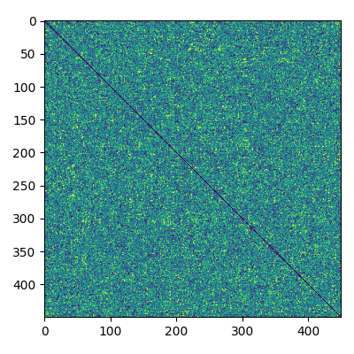
corr = envelope_correlation(label_ts, verbose=True)
# let's plot this matrix
fig, ax = plt.subplots(figsize=(4, 4))
ax.imshow(corr, cmap='viridis', clim=np.percentile(corr, [5, 95]))
fig.tight_layout()
Out:
Reading labels from parcellation...
   read 226 labels from /home/circleci/mne_data/MNE-brainstorm-data/bst_resting/subjects/bst_resting/label/lh.aparc_sub.annot
   read 224 labels from /home/circleci/mne_data/MNE-brainstorm-data/bst_resting/subjects/bst_resting/label/rh.aparc_sub.annot
Preparing the inverse operator for use...
    Scaled noise and source covariance from nave = 1 to nave = 1
    Created the regularized inverter
    Created an SSP operator (subspace dimension = 4)
    Created the whitener using a noise covariance matrix with rank 268 (4 small eigenvalues omitted)
    Computing noise-normalization factors (dSPM)...
[done]
Picked 272 channels from the data
Computing inverse...
    Eigenleads need to be weighted ...
Processing epoch : 1 / 10
Extracting time courses for 450 labels (mode: mean_flip)
Processing epoch : 2 / 10
Extracting time courses for 450 labels (mode: mean_flip)
Processing epoch : 3 / 10
Extracting time courses for 450 labels (mode: mean_flip)
Processing epoch : 4 / 10
Extracting time courses for 450 labels (mode: mean_flip)
Processing epoch : 5 / 10
Extracting time courses for 450 labels (mode: mean_flip)
Processing epoch : 6 / 10
Extracting time courses for 450 labels (mode: mean_flip)
Processing epoch : 7 / 10
Extracting time courses for 450 labels (mode: mean_flip)
Processing epoch : 8 / 10
Extracting time courses for 450 labels (mode: mean_flip)
Processing epoch : 9 / 10
Extracting time courses for 450 labels (mode: mean_flip)
Processing epoch : 10 / 10
Extracting time courses for 450 labels (mode: mean_flip)
[done]
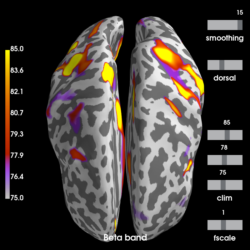
Compute the degree and plot it
threshold_prop = 0.15  # percentage of strongest edges to keep in the graph
degree = mne.connectivity.degree(corr, threshold_prop=threshold_prop)
stc = mne.labels_to_stc(labels, degree)
stc = stc.in_label(mne.Label(inv['src'][0]['vertno'], hemi='lh') +
                   mne.Label(inv['src'][1]['vertno'], hemi='rh'))
brain = stc.plot(
    clim=dict(kind='percent', lims=[75, 85, 95]), colormap='gnuplot',
    subjects_dir=subjects_dir, views='dorsal', hemi='both',
    smoothing_steps=25, time_label='Beta band')
Out:
Using control points [75. 78. 85.]
References
- 1
Joerg F Hipp, David J Hawellek, Maurizio Corbetta, Markus Siegel, and Andreas K Engel. Large-scale cortical correlation structure of spontaneous oscillatory activity. Nature Neuroscience, 15(6):884–890, 2012. doi:10.1038/nn.3101.
- 2
Sheraz Khan, Javeria A. Hashmi, Fahimeh Mamashli, Konstantinos Michmizos, Manfred G. Kitzbichler, Hari Bharadwaj, Yousra Bekhti, Santosh Ganesan, Keri-Lee A. Garel, Susan Whitfield-Gabrieli, Randy L. Gollub, Jian Kong, Lucia M. Vaina, Kunjan D. Rana, Steven M. Stufflebeam, Matti S. Hämäläinen, and Tal Kenet. Maturation trajectories of cortical resting-state networks depend on the mediating frequency band. NeuroImage, 174:57–68, 2018. doi:10.1016/j.neuroimage.2018.02.018.
Total running time of the script: ( 0 minutes 48.930 seconds)
Estimated memory usage: 911 MB