Note
Click here to download the full example code
Visualize source leakage among labels using a circular graph
This example computes all-to-all pairwise leakage among 68 regions in source space based on MNE inverse solutions and a FreeSurfer cortical parcellation. Label-to-label leakage is estimated as the correlation among the labels’ point-spread functions (PSFs). It is visualized using a circular graph which is ordered based on the locations of the regions in the axial plane.
# Authors: Olaf Hauk <olaf.hauk@mrc-cbu.cam.ac.uk>
#          Martin Luessi <mluessi@nmr.mgh.harvard.edu>
#          Alexandre Gramfort <alexandre.gramfort@inria.fr>
#          Nicolas P. Rougier (graph code borrowed from his matplotlib gallery)
#
# License: BSD (3-clause)

import numpy as np
import matplotlib.pyplot as plt

import mne
from mne.datasets import sample
from mne.minimum_norm import (read_inverse_operator,
                              make_inverse_resolution_matrix,
                              get_point_spread)

from mne.viz import circular_layout, plot_connectivity_circle

print(__doc__)
Load forward solution and inverse operator
We need a matching forward solution and inverse operator to compute resolution matrices for different methods.
data_path = sample.data_path()
subjects_dir = data_path + '/subjects'
fname_fwd = data_path + '/MEG/sample/sample_audvis-meg-eeg-oct-6-fwd.fif'
fname_inv = data_path + '/MEG/sample/sample_audvis-meg-oct-6-meg-fixed-inv.fif'
forward = mne.read_forward_solution(fname_fwd)
# Convert forward solution to fixed source orientations
mne.convert_forward_solution(
    forward, surf_ori=True, force_fixed=True, copy=False)
inverse_operator = read_inverse_operator(fname_inv)

# Compute resolution matrices for MNE
rm_mne = make_inverse_resolution_matrix(forward, inverse_operator,
                                        method='MNE', lambda2=1. / 3.**2)
src = inverse_operator['src']
del forward, inverse_operator  # save memory
Out:
Reading forward solution from /home/circleci/mne_data/MNE-sample-data/MEG/sample/sample_audvis-meg-eeg-oct-6-fwd.fif...
    Reading a source space...
    Computing patch statistics...
    Patch information added...
    Distance information added...
    [done]
    Reading a source space...
    Computing patch statistics...
    Patch information added...
    Distance information added...
    [done]
    2 source spaces read
    Desired named matrix (kind = 3523) not available
    Read MEG forward solution (7498 sources, 306 channels, free orientations)
    Desired named matrix (kind = 3523) not available
    Read EEG forward solution (7498 sources, 60 channels, free orientations)
    MEG and EEG forward solutions combined
    Source spaces transformed to the forward solution coordinate frame
    Average patch normals will be employed in the rotation to the local surface coordinates....
    Converting to surface-based source orientations...
    [done]
Reading inverse operator decomposition from /home/circleci/mne_data/MNE-sample-data/MEG/sample/sample_audvis-meg-oct-6-meg-fixed-inv.fif...
    Reading inverse operator info...
    [done]
    Reading inverse operator decomposition...
    [done]
    305 x 305 full covariance (kind = 1) found.
    Read a total of 4 projection items:
        PCA-v1 (1 x 10²) active
        PCA-v2 (1 x 10²) active
        PCA-v3 (1 x 10²) active
        Average EEG reference (1 x 60) active
    Noise covariance matrix read.
    7498 x 7498 diagonal covariance (kind = 2) found.
    Source covariance matrix read.
    Did not find the desired covariance matrix (kind = 6)
    7498 x 7498 diagonal covariance (kind = 5) found.
    Depth priors read.
    Did not find the desired covariance matrix (kind = 3)
    Reading a source space...
    Computing patch statistics...
    Patch information added...
    Distance information added...
    [done]
    Reading a source space...
    Computing patch statistics...
    Patch information added...
    Distance information added...
    [done]
    2 source spaces read
    Read a total of 4 projection items:
        PCA-v1 (1 x 10²) active
        PCA-v2 (1 x 10²) active
        PCA-v3 (1 x 10²) active
        Average EEG reference (1 x 60) active
    Source spaces transformed to the inverse solution coordinate frame
    305 out of 366 channels remain after picking
Preparing the inverse operator for use...
    Scaled noise and source covariance from nave = 1 to nave = 1
    Created the regularized inverter
    Created an SSP operator (subspace dimension = 3)
    Created the whitener using a noise covariance matrix with rank 302 (3 small eigenvalues omitted)
Applying inverse operator to ""...
    Picked 305 channels from the data
    Computing inverse...
    Eigenleads need to be weighted ...
    Computing residual...
    Explained  44.6% variance
[done]
Dimension of Inverse Matrix: (7498, 305)
Dimensions of resolution matrix: 7498 by 7498.
Read and organise labels for cortical parcellation
Get labels for FreeSurfer ‘aparc’ cortical parcellation with 34 labels/hemi
labels = mne.read_labels_from_annot('sample', parc='aparc',
                                    subjects_dir=subjects_dir)
n_labels = len(labels)
label_colors = [label.color for label in labels]
# First, we reorder the labels based on their location in the left hemi
label_names = [label.name for label in labels]
lh_labels = [name for name in label_names if name.endswith('lh')]

# Get the y-location of the label
label_ypos = list()
for name in lh_labels:
    idx = label_names.index(name)
    ypos = np.mean(labels[idx].pos[:, 1])
    label_ypos.append(ypos)

# Reorder the labels based on their location
lh_labels = [label for (yp, label) in sorted(zip(label_ypos, lh_labels))]

# For the right hemi
rh_labels = [label[:-2] + 'rh' for label in lh_labels]
Out:
Reading labels from parcellation...
   read 34 labels from /home/circleci/mne_data/MNE-sample-data/subjects/sample/label/lh.aparc.annot
   read 34 labels from /home/circleci/mne_data/MNE-sample-data/subjects/sample/label/rh.aparc.annot
Compute point-spread function summaries (PCA) for all labels
We summarise the PSFs per label by their first five principal components, and use the first component to evaluate label-to-label leakage below.
# Compute first PCA component across PSFs within labels.
# Note the differences in explained variance, probably due to different
# spatial extents of labels.
n_comp = 5
stcs_psf_mne, pca_vars_mne = get_point_spread(
    rm_mne, src, labels, mode='pca', n_comp=n_comp, norm=None,
    return_pca_vars=True)
n_verts = rm_mne.shape[0]
del rm_mne
We can show the explained variances of principal components per label. Note how they differ across labels, most likely due to their varying spatial extent.
with np.printoptions(precision=1):
    for [name, var] in zip(label_names, pca_vars_mne):
        print(f'{name}: {var.sum():.1f}% {var}')
Out:
bankssts-lh: 94.1% [41.1 33.4 10.8  5.4  3.5]
bankssts-rh: 94.7% [56.7 15.8 14.3  4.5  3.4]
caudalanteriorcingulate-lh: 97.9% [72.7 14.8  5.2  3.5  1.7]
caudalanteriorcingulate-rh: 96.8% [63.4 18.7  9.3  3.   2.4]
caudalmiddlefrontal-lh: 91.8% [35.7 25.5 14.9  8.2  7.4]
caudalmiddlefrontal-rh: 90.3% [30.2 27.5 15.9  9.3  7.3]
cuneus-lh: 95.1% [40.6 28.9 17.1  5.7  2.8]
cuneus-rh: 94.4% [39.1 32.5 15.8  3.8  3.3]
entorhinal-lh: 98.6% [52.6 27.5 10.2  6.3  2.1]
entorhinal-rh: 99.6% [48.8 37.1 12.2  0.9  0.6]
frontalpole-lh: 99.9% [70.  22.8  3.5  3.1  0.5]
frontalpole-rh: 99.8% [69.1 24.8  3.3  2.1  0.6]
fusiform-lh: 89.4% [37.9 23.  16.4  6.7  5.4]
fusiform-rh: 88.8% [32.1 28.5 15.6  6.9  5.7]
inferiorparietal-lh: 79.8% [24.1 19.1 16.9 11.2  8.5]
inferiorparietal-rh: 79.5% [24.5 17.6 16.  11.8  9.7]
inferiortemporal-lh: 85.2% [27.  22.9 15.8 11.9  7.8]
inferiortemporal-rh: 87.4% [31.8 23.2 16.3  8.4  7.7]
insula-lh: 89.9% [34.7 29.1 12.4  9.6  4. ]
insula-rh: 91.8% [39.9 26.  11.9 10.5  3.5]
isthmuscingulate-lh: 98.1% [50.4 35.3  6.1  3.9  2.4]
isthmuscingulate-rh: 97.8% [48.6 36.   7.6  3.6  2.1]
lateraloccipital-lh: 83.5% [26.4 21.  15.6 12.4  8.1]
lateraloccipital-rh: 79.4% [23.6 22.  15.1 11.1  7.6]
lateralorbitofrontal-lh: 94.2% [46.8 24.3 10.3  7.4  5.4]
lateralorbitofrontal-rh: 94.8% [44.6 26.1 13.9  5.9  4.3]
lingual-lh: 95.7% [46.8 29.5  9.5  7.8  2. ]
lingual-rh: 95.3% [53.5 27.7  7.7  4.   2.4]
medialorbitofrontal-lh: 91.8% [46.1 23.1 13.5  4.6  4.4]
medialorbitofrontal-rh: 96.5% [58.5 18.3 13.6  3.9  2.1]
middletemporal-lh: 79.5% [30.8 16.4 14.7 10.3  7.4]
middletemporal-rh: 78.9% [30.9 15.9 14.9  9.5  7.8]
paracentral-lh: 95.1% [36.6 35.2 12.8  7.3  3.2]
paracentral-rh: 93.3% [37.2 29.7 11.6 11.   3.7]
parahippocampal-lh: 96.9% [49.5 30.  11.9  3.2  2.4]
parahippocampal-rh: 98.8% [69.4 16.2  9.8  2.6  0.9]
parsopercularis-lh: 93.9% [38.8 34.  11.1  5.5  4.5]
parsopercularis-rh: 95.6% [37.6 33.8 14.9  5.   4.3]
parsorbitalis-lh: 97.5% [51.8 27.2 12.2  4.3  1.9]
parsorbitalis-rh: 98.1% [56.3 25.3  9.5  4.7  2.3]
parstriangularis-lh: 96.6% [54.1 25.7 11.3  3.1  2.5]
parstriangularis-rh: 96.1% [39.6 34.3 13.   6.5  2.6]
pericalcarine-lh: 95.7% [42.5 34.4  9.1  6.4  3.3]
pericalcarine-rh: 95.4% [44.6 34.8  9.1  4.   3. ]
postcentral-lh: 67.3% [16.7 14.5 13.4 12.8 10. ]
postcentral-rh: 65.8% [17.2 14.2 13.5 11.4  9.5]
posteriorcingulate-lh: 98.0% [54.7 31.   7.4  3.3  1.6]
posteriorcingulate-rh: 97.9% [58.4 25.   9.1  3.5  1.8]
precentral-lh: 64.3% [17.8 14.2 12.5 10.7  9.2]
precentral-rh: 63.0% [18.  14.1 11.2 10.8  8.9]
precuneus-lh: 90.5% [43.9 22.9 11.7  6.3  5.7]
precuneus-rh: 84.2% [27.2 25.9 17.1  8.2  5.9]
rostralanteriorcingulate-lh: 97.2% [53.6 22.9 12.4  5.4  2.9]
rostralanteriorcingulate-rh: 98.0% [53.6 25.2 12.2  4.9  2.1]
rostralmiddlefrontal-lh: 69.0% [17.7 15.2 14.7 11.5  9.8]
rostralmiddlefrontal-rh: 70.2% [19.7 15.5 14.3 10.7  9.9]
superiorfrontal-lh: 62.5% [16.1 15.  13.3  9.3  8.8]
superiorfrontal-rh: 61.9% [16.9 14.4 12.8  9.2  8.5]
superiorparietal-lh: 68.3% [18.4 15.2 14.6 11.2  8.9]
superiorparietal-rh: 67.2% [20.3 15.4 12.7 10.3  8.7]
superiortemporal-lh: 86.2% [29.1 19.3 15.9 14.6  7.4]
superiortemporal-rh: 86.3% [29.1 22.  16.2 12.6  6.4]
supramarginal-lh: 84.1% [28.2 21.9 15.9  9.5  8.7]
supramarginal-rh: 85.0% [28.2 22.4 16.7  9.3  8.4]
temporalpole-lh: 98.7% [53.8 33.6  6.8  3.8  0.8]
temporalpole-rh: 99.5% [76.8 16.8  4.5  0.9  0.6]
transversetemporal-lh: 99.0% [76.4 14.9  5.   1.8  1. ]
transversetemporal-rh: 98.4% [50.6 36.5  7.1  2.6  1.5]
The output shows the summed variance explained by the first five principal components as well as the explained variances of the individual components.
Evaluate leakage based on label-to-label PSF correlations
Note that correlations ignore the overall amplitude of PSFs, i.e. they do not show which region will potentially be the bigger “leaker”.
# get PSFs from Source Estimate objects into matrix
psfs_mat = np.zeros([n_labels, n_verts])
# Leakage matrix for MNE, get first principal component per label
for [i, s] in enumerate(stcs_psf_mne):
    psfs_mat[i, :] = s.data[:, 0]
# Compute label-to-label leakage as Pearson correlation of PSFs
# Sign of correlation is arbitrary, so take absolute values
leakage_mne = np.abs(np.corrcoef(psfs_mat))

# Save the plot order and create a circular layout
node_order = lh_labels[::-1] + rh_labels  # mirror label order across hemis
node_angles = circular_layout(label_names, node_order, start_pos=90,
                              group_boundaries=[0, len(label_names) / 2])
# Plot the graph using node colors from the FreeSurfer parcellation. We only
# show the 200 strongest connections.
fig = plt.figure(num=None, figsize=(8, 8), facecolor='black')
plot_connectivity_circle(leakage_mne, label_names, n_lines=200,
                         node_angles=node_angles, node_colors=label_colors,
                         title='MNE Leakage', fig=fig)
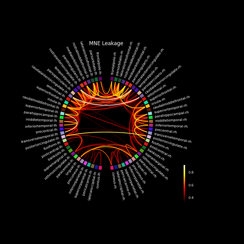
Most leakage occurs for neighbouring regions, but also for deeper regions across hemispheres.
Save the figure (optional)
Matplotlib controls figure facecolor separately for interactive display
versus for saved figures. Thus when saving you must specify facecolor,
else your labels, title, etc will not be visible:
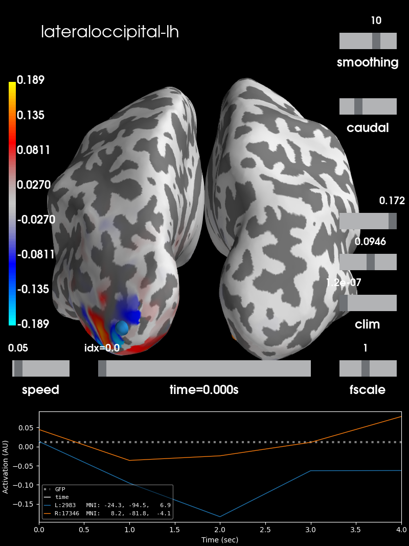
Plot PSFs for individual labels
Let us confirm for left and right lateral occipital lobes that there is indeed no leakage between them, as indicated by the correlation graph. We can plot the summary PSFs for both labels to examine the spatial extent of their leakage.
# left and right lateral occipital
idx = [22, 23]
stc_lh = stcs_psf_mne[idx[0]]
stc_rh = stcs_psf_mne[idx[1]]

# Maximum for scaling across plots
max_val = np.max([stc_lh.data, stc_rh.data])
Point-spread function for the lateral occipital label in the left hemisphere
brain_lh = stc_lh.plot(subjects_dir=subjects_dir, subject='sample',
                       hemi='both', views='caudal',
                       clim=dict(kind='value',
                                 pos_lims=(0, max_val / 2., max_val)))
brain_lh.add_text(0.1, 0.9, label_names[idx[0]], 'title', font_size=16)
and in the right hemisphere.
brain_rh = stc_rh.plot(subjects_dir=subjects_dir, subject='sample',
                       hemi='both', views='caudal',
                       clim=dict(kind='value',
                                 pos_lims=(0, max_val / 2., max_val)))
brain_rh.add_text(0.1, 0.9, label_names[idx[1]], 'title', font_size=16)
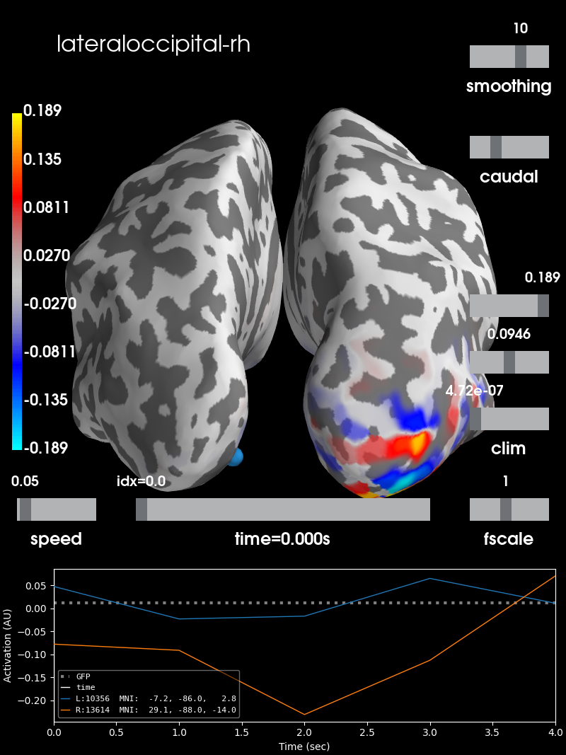
Both summary PSFs are confined to their respective hemispheres, indicating that there is indeed low leakage between these two regions.
Total running time of the script: ( 0 minutes 32.959 seconds)
Estimated memory usage: 437 MB