Note
Click here to download the full example code
Computing source space SNR
This example shows how to compute and plot source space SNR as in 1.
# Author: Padma Sundaram <tottochan@gmail.com>
# Kaisu Lankinen <klankinen@mgh.harvard.edu>
#
# License: BSD (3-clause)
import mne
from mne.datasets import sample
from mne.minimum_norm import make_inverse_operator, apply_inverse
import numpy as np
import matplotlib.pyplot as plt
print(__doc__)
data_path = sample.data_path()
subjects_dir = data_path + '/subjects'
# Read data
fname_evoked = data_path + '/MEG/sample/sample_audvis-ave.fif'
evoked = mne.read_evokeds(fname_evoked, condition='Left Auditory',
baseline=(None, 0))
fname_fwd = data_path + '/MEG/sample/sample_audvis-meg-eeg-oct-6-fwd.fif'
fname_cov = data_path + '/MEG/sample/sample_audvis-cov.fif'
fwd = mne.read_forward_solution(fname_fwd)
cov = mne.read_cov(fname_cov)
# Read inverse operator:
inv_op = make_inverse_operator(evoked.info, fwd, cov, fixed=True, verbose=True)
# Calculate MNE:
snr = 3.0
lambda2 = 1.0 / snr ** 2
stc = apply_inverse(evoked, inv_op, lambda2, 'MNE', verbose=True)
# Calculate SNR in source space:
snr_stc = stc.estimate_snr(evoked.info, fwd, cov)
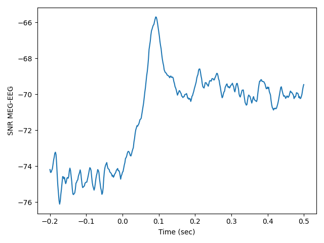
# Plot an average SNR across source points over time:
ave = np.mean(snr_stc.data, axis=0)
fig, ax = plt.subplots()
ax.plot(evoked.times, ave)
ax.set(xlabel='Time (sec)', ylabel='SNR MEG-EEG')
fig.tight_layout()
# Find time point of maximum SNR
maxidx = np.argmax(ave)
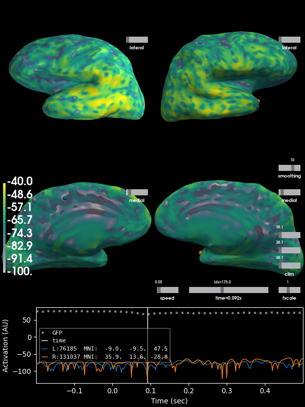
# Plot SNR on source space at the time point of maximum SNR:
kwargs = dict(initial_time=evoked.times[maxidx], hemi='split',
views=['lat', 'med'], subjects_dir=subjects_dir, size=(600, 600),
clim=dict(kind='value', lims=(-100, -70, -40)),
transparent=True, colormap='viridis')
brain = snr_stc.plot(**kwargs)
Out:
Reading /home/circleci/mne_data/MNE-sample-data/MEG/sample/sample_audvis-ave.fif ...
    Read a total of 4 projection items:
        PCA-v1 (1 x 10²) active
        PCA-v2 (1 x 10²) active
        PCA-v3 (1 x 10²) active
        Average EEG reference (1 x 60) active
    Found the data of interest:
        t =    -199.80 ...     499.49 ms (Left Auditory)
        0 CTF compensation matrices available
        nave = 55 - aspect type = 100
Projections have already been applied. Setting proj attribute to True.
Applying baseline correction (mode: mean)
Reading forward solution from /home/circleci/mne_data/MNE-sample-data/MEG/sample/sample_audvis-meg-eeg-oct-6-fwd.fif...
    Reading a source space...
    Computing patch statistics...
    Patch information added...
    Distance information added...
    [done]
    Reading a source space...
    Computing patch statistics...
    Patch information added...
    Distance information added...
    [done]
    2 source spaces read
    Desired named matrix (kind = 3523) not available
    Read MEG forward solution (7498 sources, 306 channels, free orientations)
    Desired named matrix (kind = 3523) not available
    Read EEG forward solution (7498 sources, 60 channels, free orientations)
    MEG and EEG forward solutions combined
    Source spaces transformed to the forward solution coordinate frame
    366 x 366 full covariance (kind = 1) found.
    Read a total of 4 projection items:
        PCA-v1 (1 x 10²) active
        PCA-v2 (1 x 10²) active
        PCA-v3 (1 x 10²) active
        Average EEG reference (1 x 60) active
Computing inverse operator with 364 channels.
    364 out of 366 channels remain after picking
Selected 364 channels
Creating the depth weighting matrix...
    203 planar channels
    limit = 7262/7498 = 10.020866
    scale = 2.58122e-08 exp = 0.8
    Picked elements from a free-orientation depth-weighting prior into the fixed-orientation one
    Average patch normals will be employed in the rotation to the local surface coordinates....
    Converting to surface-based source orientations...
    [done]
Whitening the forward solution.
    Created an SSP operator (subspace dimension = 4)
Computing rank from covariance with rank=None
    Using tolerance 3.3e-13 (2.2e-16 eps * 305 dim * 4.8  max singular value)
    Estimated rank (mag + grad): 302
    MEG: rank 302 computed from 305 data channels with 3 projectors
    Using tolerance 4.7e-14 (2.2e-16 eps * 59 dim * 3.6  max singular value)
    Estimated rank (eeg): 58
    EEG: rank 58 computed from 59 data channels with 1 projector
    Setting small MEG eigenvalues to zero (without PCA)
    Setting small EEG eigenvalues to zero (without PCA)
Creating the source covariance matrix
Adjusting source covariance matrix.
Computing SVD of whitened and weighted lead field matrix.
    largest singular value = 5.70263
    scaling factor to adjust the trace = 1.18949e+19
Preparing the inverse operator for use...
    Scaled noise and source covariance from nave = 1 to nave = 55
    Created the regularized inverter
    Created an SSP operator (subspace dimension = 4)
    Created the whitener using a noise covariance matrix with rank 360 (4 small eigenvalues omitted)
Applying inverse operator to "Left Auditory"...
    Picked 364 channels from the data
    Computing inverse...
    Eigenleads need to be weighted ...
    Computing residual...
    Explained  64.5% variance
[done]
    Average patch normals will be employed in the rotation to the local surface coordinates....
    Converting to surface-based source orientations...
    [done]
Computing inverse operator with 364 channels.
    364 out of 366 channels remain after picking
Selected 364 channels
    Average patch normals will be employed in the rotation to the local surface coordinates....
    Converting to surface-based source orientations...
    [done]
Whitening the forward solution.
    Created an SSP operator (subspace dimension = 4)
Computing rank from covariance with rank=None
    Using tolerance 3.3e-13 (2.2e-16 eps * 305 dim * 4.8  max singular value)
    Estimated rank (mag + grad): 302
    MEG: rank 302 computed from 305 data channels with 3 projectors
    Using tolerance 4.7e-14 (2.2e-16 eps * 59 dim * 3.6  max singular value)
    Estimated rank (eeg): 58
    EEG: rank 58 computed from 59 data channels with 1 projector
    Setting small MEG eigenvalues to zero (without PCA)
    Setting small EEG eigenvalues to zero (without PCA)
Creating the source covariance matrix
Adjusting source covariance matrix.
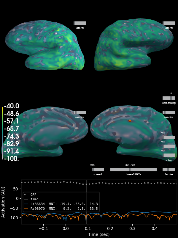
EEG
Next we do the same for EEG and plot the result on the cortex:
evoked_eeg = evoked.copy().pick_types(eeg=True, meg=False)
inv_op_eeg = make_inverse_operator(evoked_eeg.info, fwd, cov, fixed=True,
                                   verbose=True)
stc_eeg = apply_inverse(evoked_eeg, inv_op_eeg, lambda2, 'MNE', verbose=True)
snr_stc_eeg = stc_eeg.estimate_snr(evoked_eeg.info, fwd, cov)
brain = snr_stc_eeg.plot(**kwargs)
Out:
Removing projector <Projection | PCA-v1, active : True, n_channels : 102>
Removing projector <Projection | PCA-v2, active : True, n_channels : 102>
Removing projector <Projection | PCA-v3, active : True, n_channels : 102>
info["bads"] and noise_cov["bads"] do not match, excluding bad channels from both
Computing inverse operator with 59 channels.
    59 out of 366 channels remain after picking
Selected 59 channels
Creating the depth weighting matrix...
    59 EEG channels
    limit = 7499/7498 = 2.118742
    scale = 155292 exp = 0.8
    Picked elements from a free-orientation depth-weighting prior into the fixed-orientation one
    Average patch normals will be employed in the rotation to the local surface coordinates....
    Converting to surface-based source orientations...
    [done]
Whitening the forward solution.
    Created an SSP operator (subspace dimension = 1)
Computing rank from covariance with rank=None
    Using tolerance 4.7e-14 (2.2e-16 eps * 59 dim * 3.6  max singular value)
    Estimated rank (eeg): 58
    EEG: rank 58 computed from 59 data channels with 1 projector
    Setting small EEG eigenvalues to zero (without PCA)
Creating the source covariance matrix
Adjusting source covariance matrix.
Computing SVD of whitened and weighted lead field matrix.
    largest singular value = 2.81981
    scaling factor to adjust the trace = 3.0644e+19
Preparing the inverse operator for use...
    Scaled noise and source covariance from nave = 1 to nave = 55
    Created the regularized inverter
    Created an SSP operator (subspace dimension = 1)
    Created the whitener using a noise covariance matrix with rank 58 (1 small eigenvalues omitted)
Applying inverse operator to "Left Auditory"...
    Picked 59 channels from the data
    Computing inverse...
    Eigenleads need to be weighted ...
    Computing residual...
    Explained  84.4% variance
[done]
    Average patch normals will be employed in the rotation to the local surface coordinates....
    Converting to surface-based source orientations...
    [done]
info["bads"] and noise_cov["bads"] do not match, excluding bad channels from both
Computing inverse operator with 59 channels.
    59 out of 366 channels remain after picking
Selected 59 channels
    Average patch normals will be employed in the rotation to the local surface coordinates....
    Converting to surface-based source orientations...
    [done]
Whitening the forward solution.
    Created an SSP operator (subspace dimension = 1)
Computing rank from covariance with rank=None
    Using tolerance 4.7e-14 (2.2e-16 eps * 59 dim * 3.6  max singular value)
    Estimated rank (eeg): 58
    EEG: rank 58 computed from 59 data channels with 1 projector
    Setting small EEG eigenvalues to zero (without PCA)
Creating the source covariance matrix
Adjusting source covariance matrix.
The same can be done for MEG, which looks more similar to the MEG-EEG case than the EEG case does.
References
- 1
Daniel M. Goldenholz, Seppo P. Ahlfors, Matti S. Hämäläinen, Dahlia Sharon, Mamiko Ishitobi, Lucia M. Vaina, and Steven M. Stufflebeam. Mapping the signal-to-noise-ratios of cortical sources in magnetoencephalography and electroencephalography. Human Brain Mapping, 30(4):1077–1086, 2009. doi:10.1002/hbm.20571.
Total running time of the script: ( 0 minutes 27.818 seconds)
Estimated memory usage: 272 MB