How to convert 3D electrode positions to a 2D image.¶

Sometimes we want to convert a 3D representation of electrodes into a 2D image. For example, if we are using electrocorticography it is common to create scatterplots on top of a brain, with each point representing an electrode.

In this example, we’ll show two ways of doing this in MNE-Python. First, if we have the 3D locations of each electrode then we can use Mayavi to take a snapshot of a view of the brain. If we do not have these 3D locations, and only have a 2D image of the electrodes on the brain, we can use the mne.viz.ClickableImage class to choose our own electrode positions on the image.

# Authors: Christopher Holdgraf <choldgraf@berkeley.edu>
#
# License: BSD (3-clause)
from scipy.io import loadmat
import numpy as np
from matplotlib import pyplot as plt
from os import path as op

import mne
from mne.viz import ClickableImage  # noqa
from mne.viz import (plot_alignment, snapshot_brain_montage,
                     set_3d_view)


print(__doc__)

subjects_dir = mne.datasets.sample.data_path() + '/subjects'
path_data = mne.datasets.misc.data_path() + '/ecog/sample_ecog.mat'

# We've already clicked and exported
layout_path = op.join(op.dirname(mne.__file__), 'data', 'image')
layout_name = 'custom_layout.lout'

Load data¶

First we will load a sample ECoG dataset which we’ll use for generating a 2D snapshot.

mat = loadmat(path_data)
ch_names = mat['ch_names'].tolist()
elec = mat['elec']  # electrode coordinates in meters
# Now we make a montage stating that the sEEG contacts are in head
# coordinate system (although they are in MRI). This is compensated
# by the fact that below we do not specicty a trans file so the Head<->MRI
# transform is the identity.
montage = mne.channels.make_dig_montage(ch_pos=dict(zip(ch_names, elec)),
                                        coord_frame='head')
info = mne.create_info(ch_names, 1000., 'ecog').set_montage(montage)
print('Created %s channel positions' % len(ch_names))

Out:

Created 64 channel positions

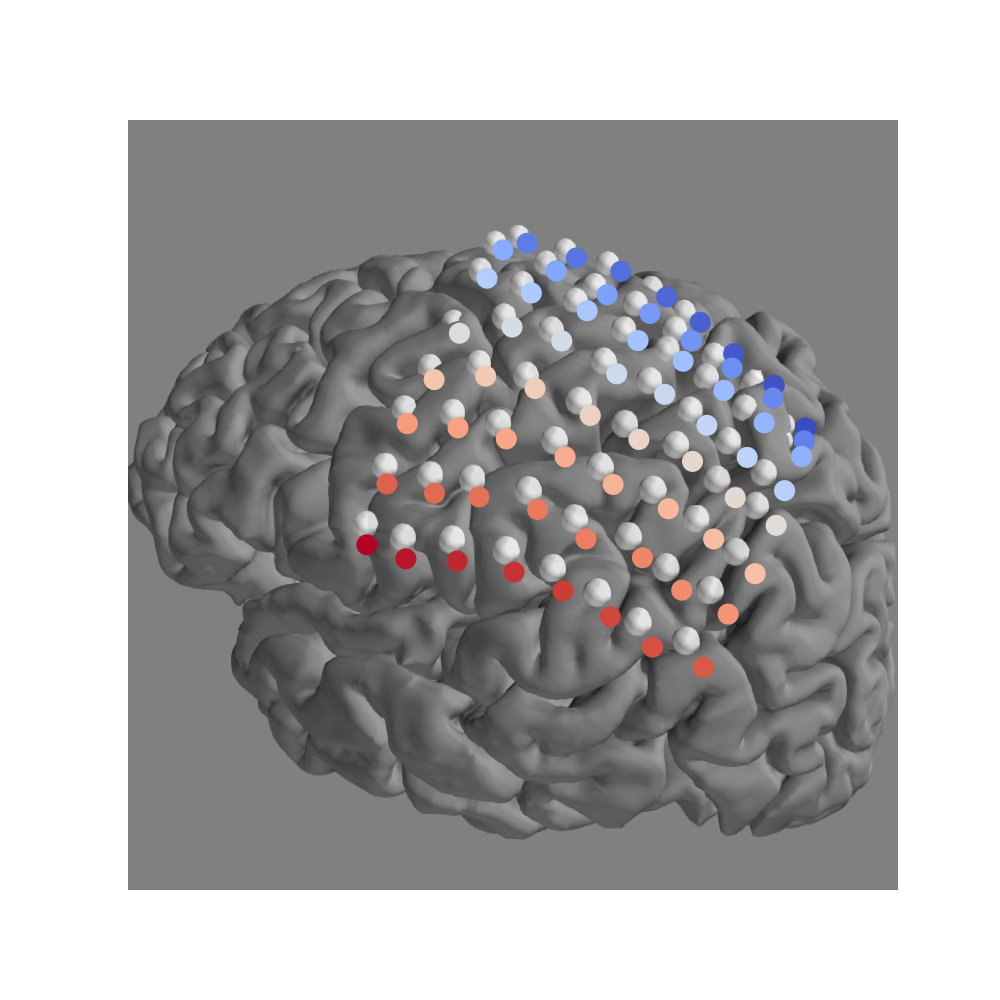
Project 3D electrodes to a 2D snapshot¶

Because we have the 3D location of each electrode, we can use the mne.viz.snapshot_brain_montage() function to return a 2D image along with the electrode positions on that image. We use this in conjunction with mne.viz.plot_alignment(), which visualizes electrode positions.

fig = plot_alignment(info, subject='sample', subjects_dir=subjects_dir,
                     surfaces=['pial'], meg=False)
set_3d_view(figure=fig, azimuth=200, elevation=70)
xy, im = snapshot_brain_montage(fig, montage)

# Convert from a dictionary to array to plot
xy_pts = np.vstack([xy[ch] for ch in info['ch_names']])

# Define an arbitrary "activity" pattern for viz
activity = np.linspace(100, 200, xy_pts.shape[0])

# This allows us to use matplotlib to create arbitrary 2d scatterplots
fig2, ax = plt.subplots(figsize=(10, 10))
ax.imshow(im)
ax.scatter(*xy_pts.T, c=activity, s=200, cmap='coolwarm')
ax.set_axis_off()
# fig2.savefig('./brain.png', bbox_inches='tight')  # For ClickableImage

Out:

Plotting 64 ECoG locations

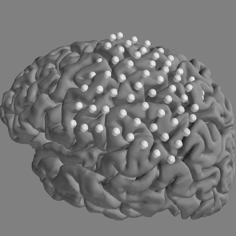
Manually creating 2D electrode positions¶

If we don’t have the 3D electrode positions then we can still create a 2D representation of the electrodes. Assuming that you can see the electrodes on the 2D image, we can use mne.viz.ClickableImage to open the image interactively. You can click points on the image and the x/y coordinate will be stored.

We’ll open an image file, then use ClickableImage to return 2D locations of mouse clicks (or load a file already created). Then, we’ll return these xy positions as a layout for use with plotting topo maps.

# This code opens the image so you can click on it. Commented out
# because we've stored the clicks as a layout file already.

# # The click coordinates are stored as a list of tuples
# im = plt.imread('./brain.png')
# click = ClickableImage(im)
# click.plot_clicks()

# # Generate a layout from our clicks and normalize by the image
# print('Generating and saving layout...')
# lt = click.to_layout()
# lt.save(op.join(layout_path, layout_name))  # To save if we want

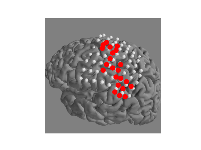
# # We've already got the layout, load it
lt = mne.channels.read_layout(layout_name, path=layout_path, scale=False)
x = lt.pos[:, 0] * float(im.shape[1])
y = (1 - lt.pos[:, 1]) * float(im.shape[0])  # Flip the y-position
fig, ax = plt.subplots()
ax.imshow(im)
ax.scatter(x, y, s=120, color='r')
plt.autoscale(tight=True)
ax.set_axis_off()
plt.show()