Plotting topographic maps of evoked data

Load evoked data and plot topomaps for selected time points using multiple additional options.

# Authors: Christian Brodbeck <christianbrodbeck@nyu.edu>
#          Tal Linzen <linzen@nyu.edu>
#          Denis A. Engeman <denis.engemann@gmail.com>
#          Mikołaj Magnuski <mmagnuski@swps.edu.pl>
#          Eric Larson <larson.eric.d@gmail.com>
#
# License: BSD (3-clause)

import numpy as np
import matplotlib.pyplot as plt

from mne.datasets import sample
from mne import read_evokeds

print(__doc__)

path = sample.data_path()
fname = path + '/MEG/sample/sample_audvis-ave.fif'

# load evoked corresponding to a specific condition
# from the fif file and subtract baseline
condition = 'Left Auditory'
evoked = read_evokeds(fname, condition=condition, baseline=(None, 0))

Out:

Reading /home/circleci/mne_data/MNE-sample-data/MEG/sample/sample_audvis-ave.fif ...
    Read a total of 4 projection items:
        PCA-v1 (1 x 102) active
        PCA-v2 (1 x 102) active
        PCA-v3 (1 x 102) active
        Average EEG reference (1 x 60) active
    Found the data of interest:
        t =    -199.80 ...     499.49 ms (Left Auditory)
        0 CTF compensation matrices available
        nave = 55 - aspect type = 100
Projections have already been applied. Setting proj attribute to True.
Applying baseline correction (mode: mean)

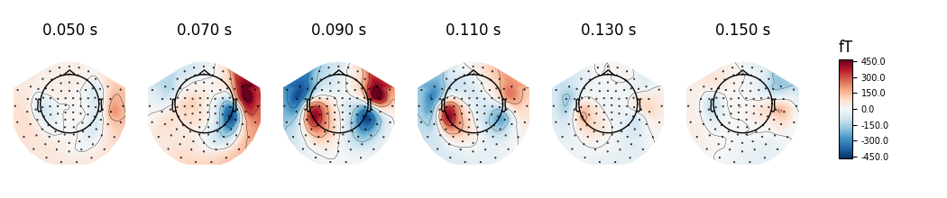
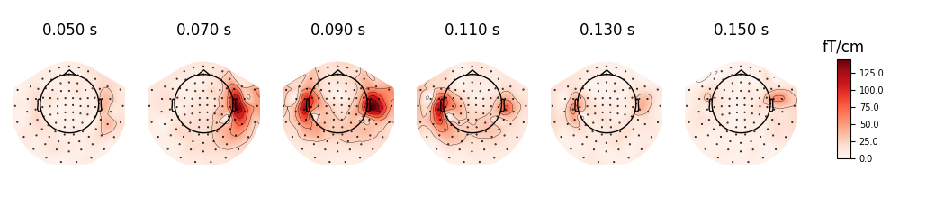
Basic plot_topomap() options

We plot evoked topographies using mne.Evoked.plot_topomap(). The first argument, times allows to specify time instants (in seconds!) for which topographies will be shown. We select timepoints from 50 to 150 ms with a step of 20ms and plot magnetometer data:

times = np.arange(0.05, 0.151, 0.02)
evoked.plot_topomap(times, ch_type='mag', time_unit='s')

Out:

Removing projector <Projection | Average EEG reference, active : True, n_channels : 60>

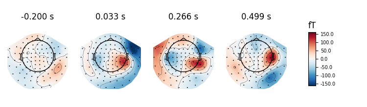
If times is set to None at most 10 regularly spaced topographies will be shown:

evoked.plot_topomap(ch_type='mag', time_unit='s')

Out:

Removing projector <Projection | Average EEG reference, active : True, n_channels : 60>

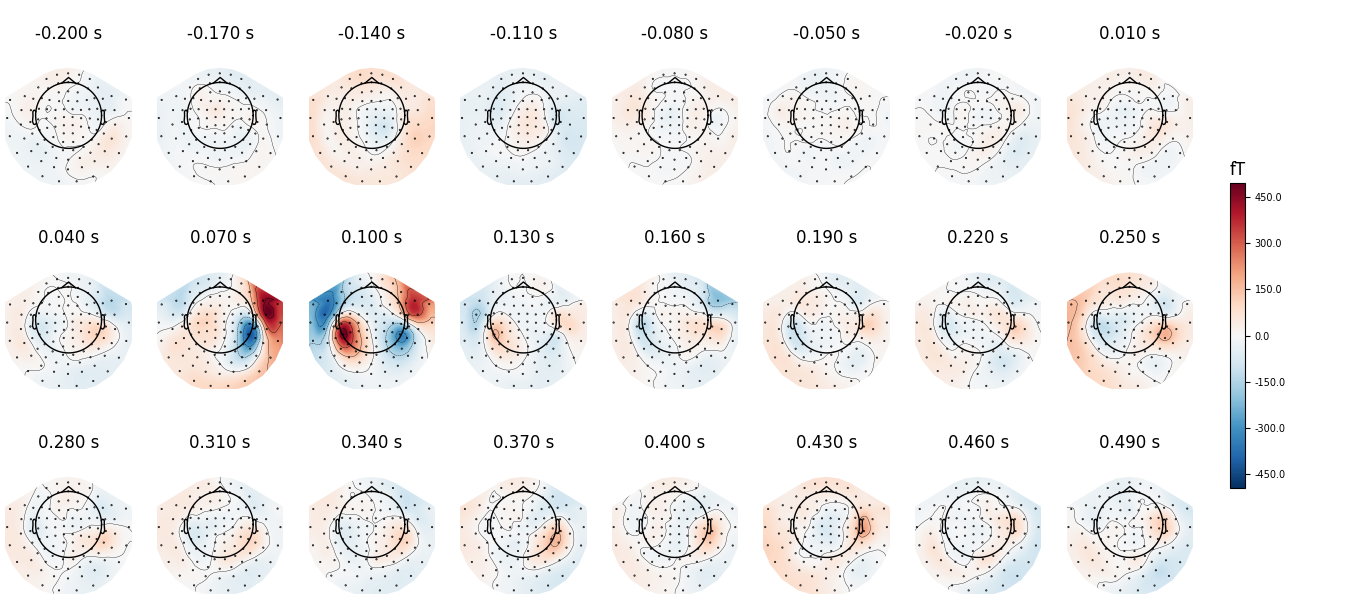
We can use nrows and ncols parameter to create multiline plots with more timepoints.

all_times = np.arange(-0.2, 0.5, 0.03)
evoked.plot_topomap(all_times, ch_type='mag', time_unit='s',
                    ncols=8, nrows='auto')

Out:

Removing projector <Projection | Average EEG reference, active : True, n_channels : 60>

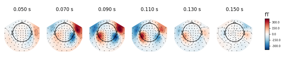
Instead of showing topographies at specific time points we can compute averages of 50 ms bins centered on these time points to reduce the noise in the topographies:

evoked.plot_topomap(times, ch_type='mag', average=0.05, time_unit='s')

Out:

Removing projector <Projection | Average EEG reference, active : True, n_channels : 60>

We can plot gradiometer data (plots the RMS for each pair of gradiometers)

evoked.plot_topomap(times, ch_type='grad', time_unit='s')

Out:

Removing projector <Projection | PCA-v1, active : True, n_channels : 102>
Removing projector <Projection | PCA-v2, active : True, n_channels : 102>
Removing projector <Projection | PCA-v3, active : True, n_channels : 102>
Removing projector <Projection | Average EEG reference, active : True, n_channels : 60>

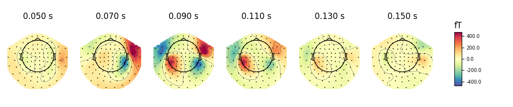
Additional plot_topomap() options

We can also use a range of various mne.viz.plot_topomap() arguments that control how the topography is drawn. For example:

• cmap - to specify the color map

• res - to control the resolution of the topographies (lower resolution means faster plotting)

• outlines='skirt' to see the topography stretched beyond the head circle

• contours to define how many contour lines should be plotted

evoked.plot_topomap(times, ch_type='mag', cmap='Spectral_r', res=32,
                    outlines='skirt', contours=4, time_unit='s')

Out:

Removing projector <Projection | Average EEG reference, active : True, n_channels : 60>

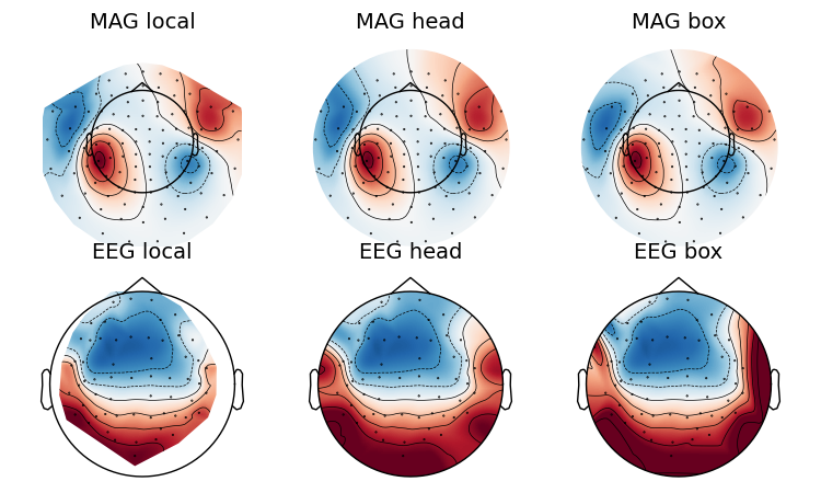
If you look at the edges of the head circle of a single topomap you’ll see the effect of extrapolation. There are three extrapolation modes:

• extrapolate='local' extrapolates only to points close to the sensors.

• extrapolate='head' extrapolates out to the head head circle.

• extrapolate='box' extrapolates to a large box stretching beyond the head circle.

The default value extrapolate='auto' will use 'local' for MEG sensors and 'head' otherwise. Here we show each option:

extrapolations = ['local', 'head', 'box']
fig, axes = plt.subplots(figsize=(7.5, 4.5), nrows=2, ncols=3)

# Here we look at EEG channels, and use a custom head sphere to get all the
# sensors to be well within the drawn head surface
for axes_row, ch_type in zip(axes, ('mag', 'eeg')):
    for ax, extr in zip(axes_row, extrapolations):
        evoked.plot_topomap(0.1, ch_type=ch_type, size=2, extrapolate=extr,
                            axes=ax, show=False, colorbar=False,
                            sphere=(0., 0., 0., 0.09))
        ax.set_title('%s %s' % (ch_type.upper(), extr), fontsize=14)
fig.tight_layout()

Out:

Removing projector <Projection | Average EEG reference, active : True, n_channels : 60>
Removing projector <Projection | Average EEG reference, active : True, n_channels : 60>
Removing projector <Projection | Average EEG reference, active : True, n_channels : 60>
Removing projector <Projection | PCA-v1, active : True, n_channels : 102>
Removing projector <Projection | PCA-v2, active : True, n_channels : 102>
Removing projector <Projection | PCA-v3, active : True, n_channels : 102>
Removing projector <Projection | PCA-v1, active : True, n_channels : 102>
Removing projector <Projection | PCA-v2, active : True, n_channels : 102>
Removing projector <Projection | PCA-v3, active : True, n_channels : 102>
Removing projector <Projection | PCA-v1, active : True, n_channels : 102>
Removing projector <Projection | PCA-v2, active : True, n_channels : 102>
Removing projector <Projection | PCA-v3, active : True, n_channels : 102>

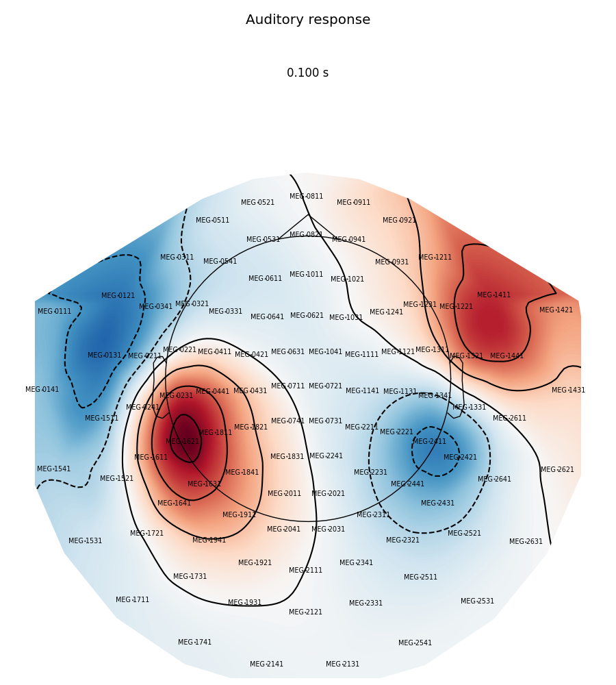
More advanced usage

Now we plot magnetometer data as topomap at a single time point: 100 ms post-stimulus, add channel labels, title and adjust plot margins:

evoked.plot_topomap(0.1, ch_type='mag', show_names=True, colorbar=False,
                    size=6, res=128, title='Auditory response',
                    time_unit='s')
plt.subplots_adjust(left=0.01, right=0.99, bottom=0.01, top=0.88)

Out:

Removing projector <Projection | Average EEG reference, active : True, n_channels : 60>

Animating the topomap

Instead of using a still image we can plot magnetometer data as an animation, which animates properly only in matplotlib interactive mode.

times = np.arange(0.05, 0.151, 0.01)
fig, anim = evoked.animate_topomap(
    times=times, ch_type='mag', frame_rate=2, time_unit='s', blit=False)

Once Loop Reflect

Estimated memory usage: 8 MB