Background information on filtering

Here we give some background information on filtering in general, and how it is done in MNE-Python in particular. Recommended reading for practical applications of digital filter design can be found in Parks & Burrus (1987) 1 and Ifeachor & Jervis (2002) 2, and for filtering in an M/EEG context we recommend reading Widmann et al. (2015) 7. To see how to use the default filters in MNE-Python on actual data, see the Filtering and resampling data tutorial.

Problem statement

Practical issues with filtering electrophysiological data are covered in Widmann et al. (2012) 6, where they conclude with this statement:

Filtering can result in considerable distortions of the time course (and amplitude) of a signal as demonstrated by VanRullen (2011) [3]. Thus, filtering should not be used lightly. However, if effects of filtering are cautiously considered and filter artifacts are minimized, a valid interpretation of the temporal dynamics of filtered electrophysiological data is possible and signals missed otherwise can be detected with filtering.

In other words, filtering can increase signal-to-noise ratio (SNR), but if it is not used carefully, it can distort data. Here we hope to cover some filtering basics so users can better understand filtering trade-offs and why MNE-Python has chosen particular defaults.

Filtering basics

Let’s get some of the basic math down. In the frequency domain, digital filters have a transfer function that is given by:

\[\begin{split}H(z) &= \frac{b_0 + b_1 z^{-1} + b_2 z^{-2} + \ldots + b_M z^{-M}} {1 + a_1 z^{-1} + a_2 z^{-2} + \ldots + a_N z^{-M}} \\ &= \frac{\sum_{k=0}^Mb_kz^{-k}}{\sum_{k=1}^Na_kz^{-k}}\end{split}\]

In the time domain, the numerator coefficients \(b_k\) and denominator coefficients \(a_k\) can be used to obtain our output data \(y(n)\) in terms of our input data \(x(n)\) as:

(1)\[\begin{split} y(n) &= b_0 x(n) + b_1 x(n-1) + \ldots + b_M x(n-M) - a_1 y(n-1) - a_2 y(n - 2) - \ldots - a_N y(n - N)\\ &= \sum_{k=0}^M b_k x(n-k) - \sum_{k=1}^N a_k y(n-k)\end{split}\]

In other words, the output at time \(n\) is determined by a sum over

1. the numerator coefficients \(b_k\), which get multiplied by the previous input values \(x(n-k)\), and

2. the denominator coefficients \(a_k\), which get multiplied by the previous output values \(y(n-k)\).

Note that these summations correspond to (1) a weighted moving average and (2) an autoregression.

Filters are broken into two classes: FIR (finite impulse response) and IIR (infinite impulse response) based on these coefficients. FIR filters use a finite number of numerator coefficients \(b_k\) (\(\forall k, a_k=0\)), and thus each output value of \(y(n)\) depends only on the \(M\) previous input values. IIR filters depend on the previous input and output values, and thus can have effectively infinite impulse responses.

As outlined in Parks & Burrus (1987) 1, FIR and IIR have different trade-offs:

• A causal FIR filter can be linear-phase – i.e., the same time delay across all frequencies – whereas a causal IIR filter cannot. The phase and group delay characteristics are also usually better for FIR filters.

• IIR filters can generally have a steeper cutoff than an FIR filter of equivalent order.

• IIR filters are generally less numerically stable, in part due to accumulating error (due to its recursive calculations).

In MNE-Python we default to using FIR filtering. As noted in Widmann et al. (2015) 7:

Despite IIR filters often being considered as computationally more efficient, they are recommended only when high throughput and sharp cutoffs are required (Ifeachor and Jervis, 2002 [2], p. 321)… FIR filters are easier to control, are always stable, have a well-defined passband, can be corrected to zero-phase without additional computations, and can be converted to minimum-phase. We therefore recommend FIR filters for most purposes in electrophysiological data analysis.

When designing a filter (FIR or IIR), there are always trade-offs that need to be considered, including but not limited to:

1. Ripple in the pass-band

2. Attenuation of the stop-band

3. Steepness of roll-off

4. Filter order (i.e., length for FIR filters)

5. Time-domain ringing

In general, the sharper something is in frequency, the broader it is in time, and vice-versa. This is a fundamental time-frequency trade-off, and it will show up below.

FIR Filters

First, we will focus on FIR filters, which are the default filters used by MNE-Python.

Designing FIR filters

Here we’ll try to design a low-pass filter and look at trade-offs in terms of time- and frequency-domain filter characteristics. Later, in Applying FIR filters, we’ll look at how such filters can affect signals when they are used.

First let’s import some useful tools for filtering, and set some default values for our data that are reasonable for M/EEG.

import numpy as np
from numpy.fft import fft, fftfreq
from scipy import signal
import matplotlib.pyplot as plt

from mne.time_frequency.tfr import morlet
from mne.viz import plot_filter, plot_ideal_filter

import mne

sfreq = 1000.
f_p = 40.
flim = (1., sfreq / 2.)  # limits for plotting

Take for example an ideal low-pass filter, which would give a magnitude response of 1 in the pass-band (up to frequency \(f_p\)) and a magnitude response of 0 in the stop-band (down to frequency \(f_s\)) such that \(f_p=f_s=40\) Hz here (shown to a lower limit of -60 dB for simplicity):

nyq = sfreq / 2.  # the Nyquist frequency is half our sample rate
freq = [0, f_p, f_p, nyq]
gain = [1, 1, 0, 0]

third_height = np.array(plt.rcParams['figure.figsize']) * [1, 1. / 3.]
ax = plt.subplots(1, figsize=third_height)[1]
plot_ideal_filter(freq, gain, ax, title='Ideal %s Hz lowpass' % f_p, flim=flim)

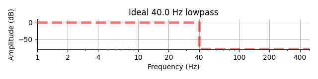
This filter hypothetically achieves zero ripple in the frequency domain, perfect attenuation, and perfect steepness. However, due to the discontinuity in the frequency response, the filter would require infinite ringing in the time domain (i.e., infinite order) to be realized. Another way to think of this is that a rectangular window in the frequency domain is actually a sinc function in the time domain, which requires an infinite number of samples (and thus infinite time) to represent. So although this filter has ideal frequency suppression, it has poor time-domain characteristics.

Let’s try to naïvely make a brick-wall filter of length 0.1 s, and look at the filter itself in the time domain and the frequency domain:

n = int(round(0.1 * sfreq))
n -= n % 2 - 1  # make it odd
t = np.arange(-(n // 2), n // 2 + 1) / sfreq  # center our sinc
h = np.sinc(2 * f_p * t) / (4 * np.pi)
plot_filter(h, sfreq, freq, gain, 'Sinc (0.1 s)', flim=flim, compensate=True)

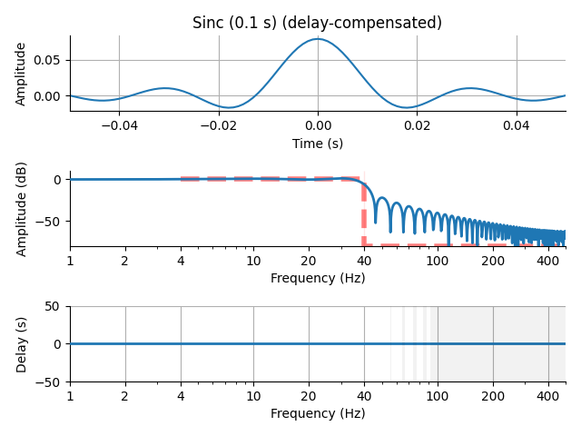
This is not so good! Making the filter 10 times longer (1 s) gets us a slightly better stop-band suppression, but still has a lot of ringing in the time domain. Note the x-axis is an order of magnitude longer here, and the filter has a correspondingly much longer group delay (again equal to half the filter length, or 0.5 seconds):

n = int(round(1. * sfreq))
n -= n % 2 - 1  # make it odd
t = np.arange(-(n // 2), n // 2 + 1) / sfreq
h = np.sinc(2 * f_p * t) / (4 * np.pi)
plot_filter(h, sfreq, freq, gain, 'Sinc (1.0 s)', flim=flim, compensate=True)

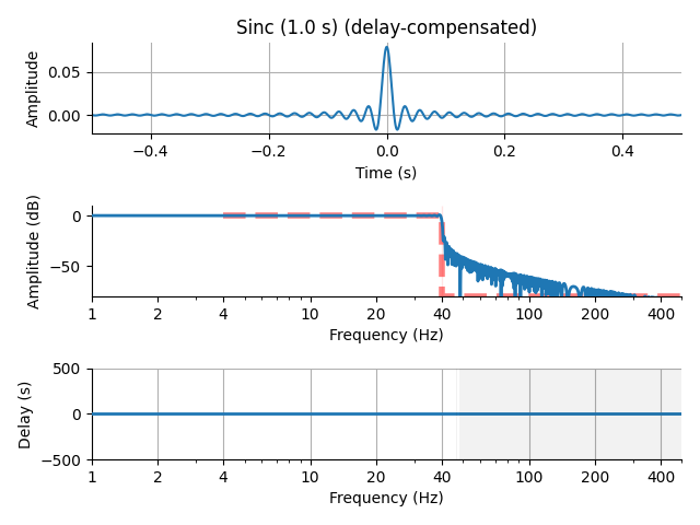
Let’s make the stop-band tighter still with a longer filter (10 s), with a resulting larger x-axis:

n = int(round(10. * sfreq))
n -= n % 2 - 1  # make it odd
t = np.arange(-(n // 2), n // 2 + 1) / sfreq
h = np.sinc(2 * f_p * t) / (4 * np.pi)
plot_filter(h, sfreq, freq, gain, 'Sinc (10.0 s)', flim=flim, compensate=True)

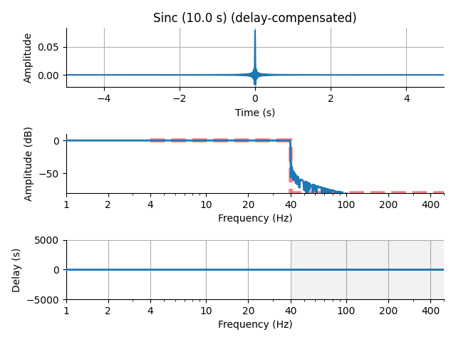
Now we have very sharp frequency suppression, but our filter rings for the entire 10 seconds. So this naïve method is probably not a good way to build our low-pass filter.

Fortunately, there are multiple established methods to design FIR filters based on desired response characteristics. These include:

1. The Remez algorithm (scipy.signal.remez(), MATLAB firpm)

2. Windowed FIR design (scipy.signal.firwin2(), scipy.signal.firwin(), and MATLAB fir2)

3. Least squares designs (scipy.signal.firls(), MATLAB firls)

4. Frequency-domain design (construct filter in Fourier domain and use an IFFT to invert it)

Note

Remez and least squares designs have advantages when there are “do not care” regions in our frequency response. However, we want well controlled responses in all frequency regions. Frequency-domain construction is good when an arbitrary response is desired, but generally less clean (due to sampling issues) than a windowed approach for more straightforward filter applications. Since our filters (low-pass, high-pass, band-pass, band-stop) are fairly simple and we require precise control of all frequency regions, we will primarily use and explore windowed FIR design.

If we relax our frequency-domain filter requirements a little bit, we can use these functions to construct a lowpass filter that instead has a transition band, or a region between the pass frequency \(f_p\) and stop frequency \(f_s\), e.g.:

trans_bandwidth = 10  # 10 Hz transition band
f_s = f_p + trans_bandwidth  # = 50 Hz

freq = [0., f_p, f_s, nyq]
gain = [1., 1., 0., 0.]
ax = plt.subplots(1, figsize=third_height)[1]
title = '%s Hz lowpass with a %s Hz transition' % (f_p, trans_bandwidth)
plot_ideal_filter(freq, gain, ax, title=title, flim=flim)

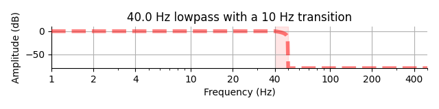
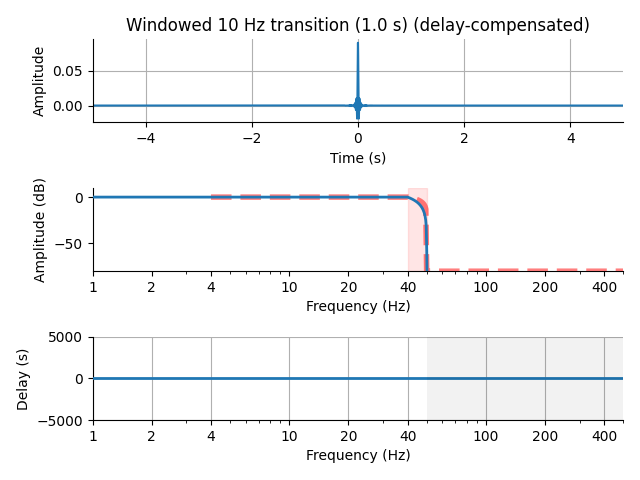
Accepting a shallower roll-off of the filter in the frequency domain makes our time-domain response potentially much better. We end up with a more gradual slope through the transition region, but a much cleaner time domain signal. Here again for the 1 s filter:

h = signal.firwin2(n, freq, gain, nyq=nyq)
plot_filter(h, sfreq, freq, gain, 'Windowed 10 Hz transition (1.0 s)',
            flim=flim, compensate=True)

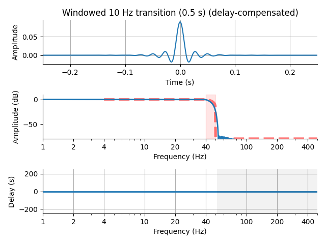
Since our lowpass is around 40 Hz with a 10 Hz transition, we can actually use a shorter filter (5 cycles at 10 Hz = 0.5 s) and still get acceptable stop-band attenuation:

n = int(round(sfreq * 0.5)) + 1
h = signal.firwin2(n, freq, gain, nyq=nyq)
plot_filter(h, sfreq, freq, gain, 'Windowed 10 Hz transition (0.5 s)',
            flim=flim, compensate=True)

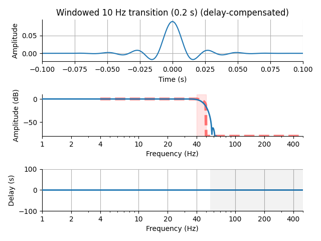
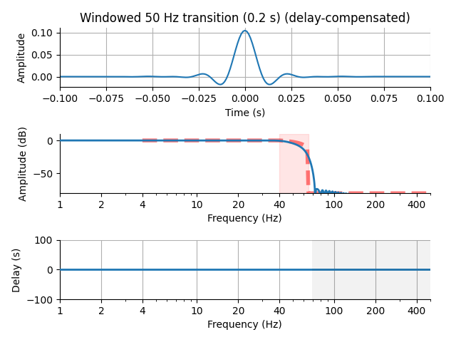
But if we shorten the filter too much (2 cycles of 10 Hz = 0.2 s), our effective stop frequency gets pushed out past 60 Hz:

n = int(round(sfreq * 0.2)) + 1
h = signal.firwin2(n, freq, gain, nyq=nyq)
plot_filter(h, sfreq, freq, gain, 'Windowed 10 Hz transition (0.2 s)',
            flim=flim, compensate=True)

If we want a filter that is only 0.1 seconds long, we should probably use something more like a 25 Hz transition band (0.2 s = 5 cycles @ 25 Hz):

trans_bandwidth = 25
f_s = f_p + trans_bandwidth
freq = [0, f_p, f_s, nyq]
h = signal.firwin2(n, freq, gain, nyq=nyq)
plot_filter(h, sfreq, freq, gain, 'Windowed 50 Hz transition (0.2 s)',
            flim=flim, compensate=True)

So far, we have only discussed non-causal filtering, which means that each sample at each time point \(t\) is filtered using samples that come after (\(t + \Delta t\)) and before (\(t - \Delta t\)) the current time point \(t\). In this sense, each sample is influenced by samples that come both before and after it. This is useful in many cases, especially because it does not delay the timing of events.

However, sometimes it can be beneficial to use causal filtering, whereby each sample \(t\) is filtered only using time points that came after it.

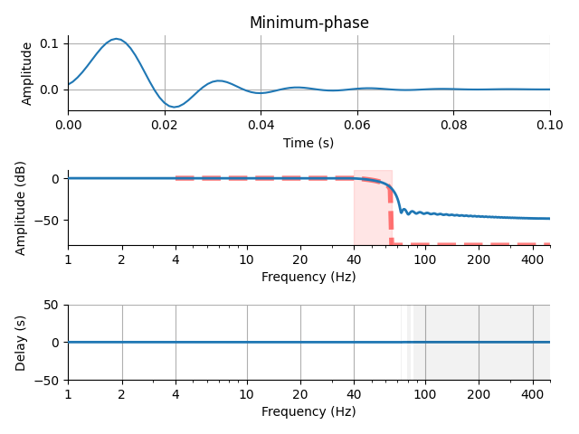
Note that the delay is variable (whereas for linear/zero-phase filters it is constant) but small in the pass-band. Unlike zero-phase filters, which require time-shifting backward the output of a linear-phase filtering stage (and thus becoming non-causal), minimum-phase filters do not require any compensation to achieve small delays in the pass-band. Note that as an artifact of the minimum phase filter construction step, the filter does not end up being as steep as the linear/zero-phase version.

We can construct a minimum-phase filter from our existing linear-phase filter with the scipy.signal.minimum_phase() function, and note that the falloff is not as steep:

h_min = signal.minimum_phase(h)
plot_filter(h_min, sfreq, freq, gain, 'Minimum-phase', flim=flim)

Applying FIR filters

Now lets look at some practical effects of these filters by applying them to some data.

Let’s construct a Gaussian-windowed sinusoid (i.e., Morlet imaginary part) plus noise (random and line). Note that the original clean signal contains frequency content in both the pass band and transition bands of our low-pass filter.

dur = 10.
center = 2.
morlet_freq = f_p
tlim = [center - 0.2, center + 0.2]
tticks = [tlim[0], center, tlim[1]]
flim = [20, 70]

x = np.zeros(int(sfreq * dur) + 1)
blip = morlet(sfreq, [morlet_freq], n_cycles=7)[0].imag / 20.
n_onset = int(center * sfreq) - len(blip) // 2
x[n_onset:n_onset + len(blip)] += blip
x_orig = x.copy()

rng = np.random.RandomState(0)
x += rng.randn(len(x)) / 1000.
x += np.sin(2. * np.pi * 60. * np.arange(len(x)) / sfreq) / 2000.

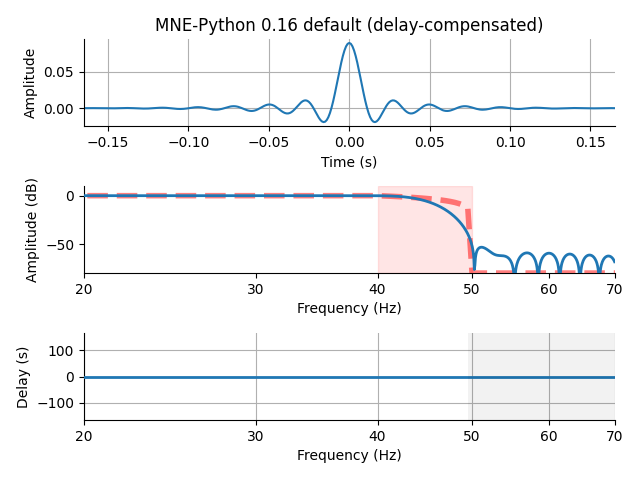
Filter it with a shallow cutoff, linear-phase FIR (which allows us to compensate for the constant filter delay):

transition_band = 0.25 * f_p
f_s = f_p + transition_band
freq = [0., f_p, f_s, sfreq / 2.]
gain = [1., 1., 0., 0.]
# This would be equivalent:
h = mne.filter.create_filter(x, sfreq, l_freq=None, h_freq=f_p,
                             fir_design='firwin', verbose=True)
x_v16 = np.convolve(h, x)
# this is the linear->zero phase, causal-to-non-causal conversion / shift
x_v16 = x_v16[len(h) // 2:]

plot_filter(h, sfreq, freq, gain, 'MNE-Python 0.16 default', flim=flim,
            compensate=True)

Out:

Setting up low-pass filter at 40 Hz

FIR filter parameters
---------------------
Designing a one-pass, zero-phase, non-causal lowpass filter:
- Windowed time-domain design (firwin) method
- Hamming window with 0.0194 passband ripple and 53 dB stopband attenuation
- Upper passband edge: 40.00 Hz
- Upper transition bandwidth: 10.00 Hz (-6 dB cutoff frequency: 45.00 Hz)
- Filter length: 331 samples (0.331 sec)

Filter it with a different design method fir_design="firwin2", and also compensate for the constant filter delay. This method does not produce quite as sharp a transition compared to fir_design="firwin", despite being twice as long:

transition_band = 0.25 * f_p
f_s = f_p + transition_band
freq = [0., f_p, f_s, sfreq / 2.]
gain = [1., 1., 0., 0.]
# This would be equivalent:
# filter_dur = 6.6 / transition_band  # sec
# n = int(sfreq * filter_dur)
# h = signal.firwin2(n, freq, gain, nyq=sfreq / 2.)
h = mne.filter.create_filter(x, sfreq, l_freq=None, h_freq=f_p,
                             fir_design='firwin2', verbose=True)
x_v14 = np.convolve(h, x)[len(h) // 2:]

plot_filter(h, sfreq, freq, gain, 'MNE-Python 0.14 default', flim=flim,
            compensate=True)

Out:

Setting up low-pass filter at 40 Hz

FIR filter parameters
---------------------
Designing a one-pass, zero-phase, non-causal lowpass filter:
- Windowed frequency-domain design (firwin2) method
- Hamming window
- Upper passband edge: 40.00 Hz
- Upper transition bandwidth: 10.00 Hz (-6 dB cutoff frequency: 45.00 Hz)
- Filter length: 661 samples (0.661 sec)

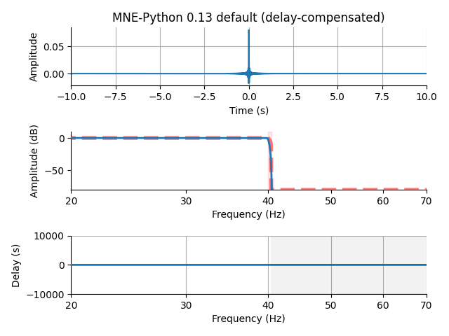
Let’s also filter with the MNE-Python 0.13 default, which is a long-duration, steep cutoff FIR that gets applied twice:

transition_band = 0.5  # Hz
f_s = f_p + transition_band
filter_dur = 10.  # sec
freq = [0., f_p, f_s, sfreq / 2.]
gain = [1., 1., 0., 0.]
# This would be equivalent
# n = int(sfreq * filter_dur)
# h = signal.firwin2(n, freq, gain, nyq=sfreq / 2.)
h = mne.filter.create_filter(x, sfreq, l_freq=None, h_freq=f_p,
                             h_trans_bandwidth=transition_band,
                             filter_length='%ss' % filter_dur,
                             fir_design='firwin2', verbose=True)
x_v13 = np.convolve(np.convolve(h, x)[::-1], h)[::-1][len(h) - 1:-len(h) - 1]
# the effective h is one that is applied to the time-reversed version of itself
h_eff = np.convolve(h, h[::-1])
plot_filter(h_eff, sfreq, freq, gain, 'MNE-Python 0.13 default', flim=flim,
            compensate=True)

Out:

Setting up low-pass filter at 40 Hz

FIR filter parameters
---------------------
Designing a one-pass, zero-phase, non-causal lowpass filter:
- Windowed frequency-domain design (firwin2) method
- Hamming window
- Upper passband edge: 40.00 Hz
- Upper transition bandwidth: 0.50 Hz (-6 dB cutoff frequency: 40.25 Hz)
- Filter length: 10001 samples (10.001 sec)

Let’s also filter it with the MNE-C default, which is a long-duration steep-slope FIR filter designed using frequency-domain techniques:

h = mne.filter.design_mne_c_filter(sfreq, l_freq=None, h_freq=f_p + 2.5)
x_mne_c = np.convolve(h, x)[len(h) // 2:]

transition_band = 5  # Hz (default in MNE-C)
f_s = f_p + transition_band
freq = [0., f_p, f_s, sfreq / 2.]
gain = [1., 1., 0., 0.]
plot_filter(h, sfreq, freq, gain, 'MNE-C default', flim=flim, compensate=True)

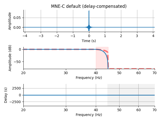
Out:

filter :   0.000 ...   42.5 Hz   bins : 0 ... 348 of 4097 hpw : 3 lpw : 20

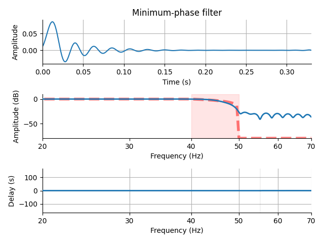
And now an example of a minimum-phase filter:

h = mne.filter.create_filter(x, sfreq, l_freq=None, h_freq=f_p,
                             phase='minimum', fir_design='firwin',
                             verbose=True)
x_min = np.convolve(h, x)
transition_band = 0.25 * f_p
f_s = f_p + transition_band
filter_dur = 6.6 / transition_band  # sec
n = int(sfreq * filter_dur)
freq = [0., f_p, f_s, sfreq / 2.]
gain = [1., 1., 0., 0.]
plot_filter(h, sfreq, freq, gain, 'Minimum-phase filter', flim=flim)

Out:

Setting up low-pass filter at 40 Hz

FIR filter parameters
---------------------
Designing a one-pass, non-linear phase, causal lowpass filter:
- Windowed time-domain design (firwin) method
- Hamming window with 0.0194 passband ripple and 53 dB stopband attenuation
- Upper transition bandwidth: 10.00 Hz
- Filter length: 331 samples (0.331 sec)

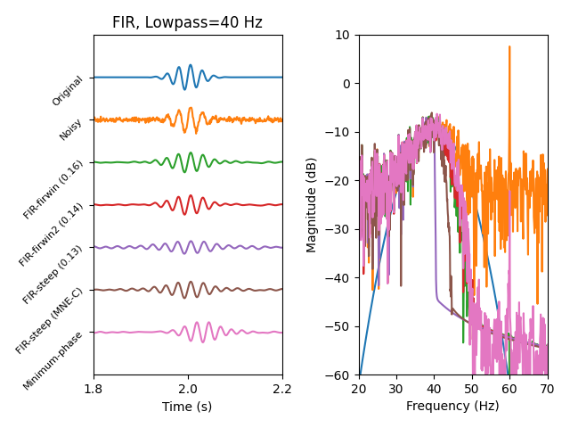
Both the MNE-Python 0.13 and MNE-C filters have excellent frequency attenuation, but it comes at a cost of potential ringing (long-lasting ripples) in the time domain. Ringing can occur with steep filters, especially in signals with frequency content around the transition band. Our Morlet wavelet signal has power in our transition band, and the time-domain ringing is thus more pronounced for the steep-slope, long-duration filter than the shorter, shallower-slope filter:

axes = plt.subplots(1, 2)[1]


def plot_signal(x, offset):
    """Plot a signal."""
    t = np.arange(len(x)) / sfreq
    axes[0].plot(t, x + offset)
    axes[0].set(xlabel='Time (s)', xlim=t[[0, -1]])
    X = fft(x)
    freqs = fftfreq(len(x), 1. / sfreq)
    mask = freqs >= 0
    X = X[mask]
    freqs = freqs[mask]
    axes[1].plot(freqs, 20 * np.log10(np.maximum(np.abs(X), 1e-16)))
    axes[1].set(xlim=flim)


yscale = 30
yticklabels = ['Original', 'Noisy', 'FIR-firwin (0.16)', 'FIR-firwin2 (0.14)',
               'FIR-steep (0.13)', 'FIR-steep (MNE-C)', 'Minimum-phase']
yticks = -np.arange(len(yticklabels)) / yscale
plot_signal(x_orig, offset=yticks[0])
plot_signal(x, offset=yticks[1])
plot_signal(x_v16, offset=yticks[2])
plot_signal(x_v14, offset=yticks[3])
plot_signal(x_v13, offset=yticks[4])
plot_signal(x_mne_c, offset=yticks[5])
plot_signal(x_min, offset=yticks[6])
axes[0].set(xlim=tlim, title='FIR, Lowpass=%d Hz' % f_p, xticks=tticks,
            ylim=[-len(yticks) / yscale, 1. / yscale],
            yticks=yticks, yticklabels=yticklabels)
for text in axes[0].get_yticklabels():
    text.set(rotation=45, size=8)
axes[1].set(xlim=flim, ylim=(-60, 10), xlabel='Frequency (Hz)',
            ylabel='Magnitude (dB)')
mne.viz.tight_layout()
plt.show()

IIR filters

MNE-Python also offers IIR filtering functionality that is based on the methods from scipy.signal. Specifically, we use the general-purpose functions scipy.signal.iirfilter() and scipy.signal.iirdesign(), which provide unified interfaces to IIR filter design.

Designing IIR filters

Let’s continue with our design of a 40 Hz low-pass filter and look at some trade-offs of different IIR filters.

Often the default IIR filter is a Butterworth filter, which is designed to have a maximally flat pass-band. Let’s look at a few filter orders, i.e., a few different number of coefficients used and therefore steepness of the filter:

Note

Notice that the group delay (which is related to the phase) of the IIR filters below are not constant. In the FIR case, we can design so-called linear-phase filters that have a constant group delay, and thus compensate for the delay (making the filter non-causal) if necessary. This cannot be done with IIR filters, as they have a non-linear phase (non-constant group delay). As the filter order increases, the phase distortion near and in the transition band worsens. However, if non-causal (forward-backward) filtering can be used, e.g. with scipy.signal.filtfilt(), these phase issues can theoretically be mitigated.

sos = signal.iirfilter(2, f_p / nyq, btype='low', ftype='butter', output='sos')
plot_filter(dict(sos=sos), sfreq, freq, gain, 'Butterworth order=2', flim=flim,
            compensate=True)
x_shallow = signal.sosfiltfilt(sos, x)
del sos

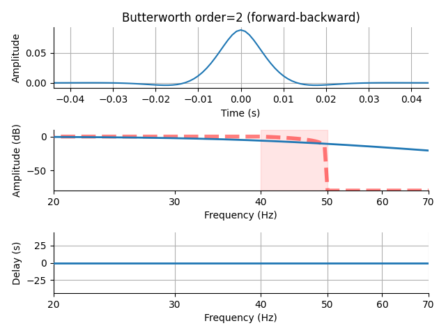
The falloff of this filter is not very steep.

Note

Here we have made use of second-order sections (SOS) by using scipy.signal.sosfilt() and, under the hood, scipy.signal.zpk2sos() when passing the output='sos' keyword argument to scipy.signal.iirfilter(). The filter definitions given above use the polynomial numerator/denominator (sometimes called “tf”) form (b, a), which are theoretically equivalent to the SOS form used here. In practice, however, the SOS form can give much better results due to issues with numerical precision (see scipy.signal.sosfilt() for an example), so SOS should be used whenever possible.

Let’s increase the order, and note that now we have better attenuation, with a longer impulse response. Let’s also switch to using the MNE filter design function, which simplifies a few things and gives us some information about the resulting filter:

iir_params = dict(order=8, ftype='butter')
filt = mne.filter.create_filter(x, sfreq, l_freq=None, h_freq=f_p,
                                method='iir', iir_params=iir_params,
                                verbose=True)
plot_filter(filt, sfreq, freq, gain, 'Butterworth order=8', flim=flim,
            compensate=True)
x_steep = signal.sosfiltfilt(filt['sos'], x)

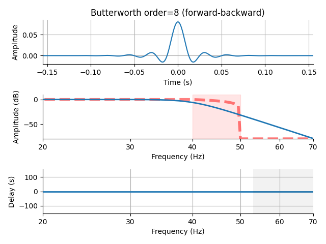
Out:

Setting up low-pass filter at 40 Hz

IIR filter parameters
---------------------
Butterworth lowpass zero-phase (two-pass forward and reverse) non-causal filter:
- Filter order 16 (effective, after forward-backward)
- Cutoff at 40.00 Hz: -6.02 dB

There are other types of IIR filters that we can use. For a complete list, check out the documentation for scipy.signal.iirdesign(). Let’s try a Chebychev (type I) filter, which trades off ripple in the pass-band to get better attenuation in the stop-band:

iir_params.update(ftype='cheby1',
                  rp=1.,  # dB of acceptable pass-band ripple
                  )
filt = mne.filter.create_filter(x, sfreq, l_freq=None, h_freq=f_p,
                                method='iir', iir_params=iir_params,
                                verbose=True)
plot_filter(filt, sfreq, freq, gain,
            'Chebychev-1 order=8, ripple=1 dB', flim=flim, compensate=True)

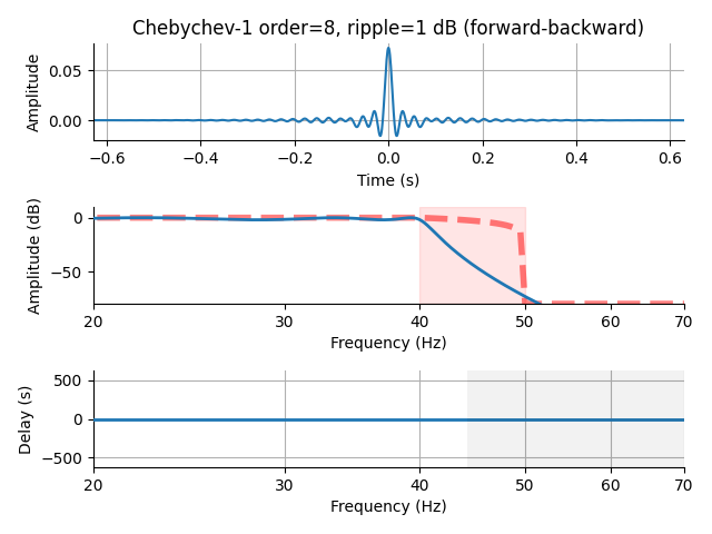
Out:

Setting up low-pass filter at 40 Hz

IIR filter parameters
---------------------
Chebyshev I lowpass zero-phase (two-pass forward and reverse) non-causal filter:
- Filter order 16 (effective, after forward-backward)
- Cutoff at 40.00 Hz: -2.00 dB

If we can live with even more ripple, we can get it slightly steeper, but the impulse response begins to ring substantially longer (note the different x-axis scale):

iir_params['rp'] = 6.
filt = mne.filter.create_filter(x, sfreq, l_freq=None, h_freq=f_p,
                                method='iir', iir_params=iir_params,
                                verbose=True)
plot_filter(filt, sfreq, freq, gain,
            'Chebychev-1 order=8, ripple=6 dB', flim=flim,
            compensate=True)

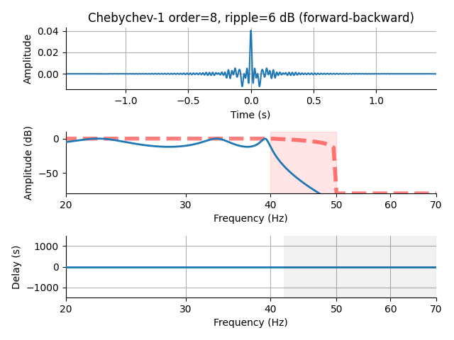
Out:

Setting up low-pass filter at 40 Hz

IIR filter parameters
---------------------
Chebyshev I lowpass zero-phase (two-pass forward and reverse) non-causal filter:
- Filter order 16 (effective, after forward-backward)
- Cutoff at 40.00 Hz: -12.00 dB

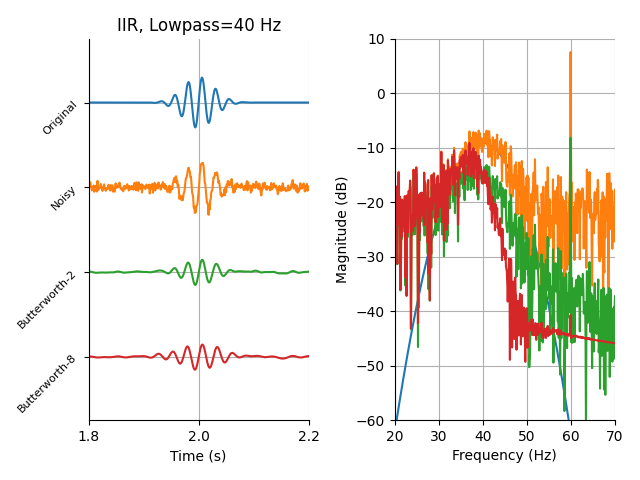
Applying IIR filters

Now let’s look at how our shallow and steep Butterworth IIR filters perform on our Morlet signal from before:

axes = plt.subplots(1, 2)[1]
yticks = np.arange(4) / -30.
yticklabels = ['Original', 'Noisy', 'Butterworth-2', 'Butterworth-8']
plot_signal(x_orig, offset=yticks[0])
plot_signal(x, offset=yticks[1])
plot_signal(x_shallow, offset=yticks[2])
plot_signal(x_steep, offset=yticks[3])
axes[0].set(xlim=tlim, title='IIR, Lowpass=%d Hz' % f_p, xticks=tticks,
            ylim=[-0.125, 0.025], yticks=yticks, yticklabels=yticklabels,)
for text in axes[0].get_yticklabels():
    text.set(rotation=45, size=8)
axes[1].set(xlim=flim, ylim=(-60, 10), xlabel='Frequency (Hz)',
            ylabel='Magnitude (dB)')
mne.viz.adjust_axes(axes)
mne.viz.tight_layout()
plt.show()

Some pitfalls of filtering

Multiple recent papers have noted potential risks of drawing errant inferences due to misapplication of filters.

Low-pass problems

Filters in general, especially those that are non-causal (zero-phase), can make activity appear to occur earlier or later than it truly did. As mentioned in VanRullen (2011) 3, investigations of commonly (at the time) used low-pass filters created artifacts when they were applied to simulated data. However, such deleterious effects were minimal in many real-world examples in Rousselet (2012) 5.

Perhaps more revealing, it was noted in Widmann & Schröger (2012) 6 that the problematic low-pass filters from VanRullen (2011) 3:

1. Used a least-squares design (like scipy.signal.firls()) that included “do-not-care” transition regions, which can lead to uncontrolled behavior.

2. Had a filter length that was independent of the transition bandwidth, which can cause excessive ringing and signal distortion.

High-pass problems

When it comes to high-pass filtering, using corner frequencies above 0.1 Hz were found in Acunzo et al. (2012) 4 to:

“… generate a systematic bias easily leading to misinterpretations of neural activity.”

In a related paper, Widmann et al. (2015) 7 also came to suggest a 0.1 Hz highpass. More evidence followed in Tanner et al. (2015) 8 of such distortions. Using data from language ERP studies of semantic and syntactic processing (i.e., N400 and P600), using a high-pass above 0.3 Hz caused significant effects to be introduced implausibly early when compared to the unfiltered data. From this, the authors suggested the optimal high-pass value for language processing to be 0.1 Hz.

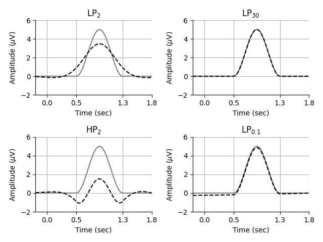
We can recreate a problematic simulation from Tanner et al. (2015) 8:

“The simulated component is a single-cycle cosine wave with an amplitude of 5µV [sic], onset of 500 ms poststimulus, and duration of 800 ms. The simulated component was embedded in 20 s of zero values to avoid filtering edge effects… Distortions [were] caused by 2 Hz low-pass and high-pass filters… No visible distortion to the original waveform [occurred] with 30 Hz low-pass and 0.01 Hz high-pass filters… Filter frequencies correspond to the half-amplitude (-6 dB) cutoff (12 dB/octave roll-off).”

Note

This simulated signal contains energy not just within the pass-band, but also within the transition and stop-bands – perhaps most easily understood because the signal has a non-zero DC value, but also because it is a shifted cosine that has been windowed (here multiplied by a rectangular window), which makes the cosine and DC frequencies spread to other frequencies (multiplication in time is convolution in frequency, so multiplying by a rectangular window in the time domain means convolving a sinc function with the impulses at DC and the cosine frequency in the frequency domain).

x = np.zeros(int(2 * sfreq))
t = np.arange(0, len(x)) / sfreq - 0.2
onset = np.where(t >= 0.5)[0][0]
cos_t = np.arange(0, int(sfreq * 0.8)) / sfreq
sig = 2.5 - 2.5 * np.cos(2 * np.pi * (1. / 0.8) * cos_t)
x[onset:onset + len(sig)] = sig

iir_lp_30 = signal.iirfilter(2, 30. / sfreq, btype='lowpass')
iir_hp_p1 = signal.iirfilter(2, 0.1 / sfreq, btype='highpass')
iir_lp_2 = signal.iirfilter(2, 2. / sfreq, btype='lowpass')
iir_hp_2 = signal.iirfilter(2, 2. / sfreq, btype='highpass')
x_lp_30 = signal.filtfilt(iir_lp_30[0], iir_lp_30[1], x, padlen=0)
x_hp_p1 = signal.filtfilt(iir_hp_p1[0], iir_hp_p1[1], x, padlen=0)
x_lp_2 = signal.filtfilt(iir_lp_2[0], iir_lp_2[1], x, padlen=0)
x_hp_2 = signal.filtfilt(iir_hp_2[0], iir_hp_2[1], x, padlen=0)

xlim = t[[0, -1]]
ylim = [-2, 6]
xlabel = 'Time (sec)'
ylabel = r'Amplitude ($\mu$V)'
tticks = [0, 0.5, 1.3, t[-1]]
axes = plt.subplots(2, 2)[1].ravel()
for ax, x_f, title in zip(axes, [x_lp_2, x_lp_30, x_hp_2, x_hp_p1],
                          ['LP$_2$', 'LP$_{30}$', 'HP$_2$', 'LP$_{0.1}$']):
    ax.plot(t, x, color='0.5')
    ax.plot(t, x_f, color='k', linestyle='--')
    ax.set(ylim=ylim, xlim=xlim, xticks=tticks,
           title=title, xlabel=xlabel, ylabel=ylabel)
mne.viz.adjust_axes(axes)
mne.viz.tight_layout()
plt.show()

Similarly, in a P300 paradigm reported by Kappenman & Luck (2010) 12, they found that applying a 1 Hz high-pass decreased the probability of finding a significant difference in the N100 response, likely because the P300 response was smeared (and inverted) in time by the high-pass filter such that it tended to cancel out the increased N100. However, they nonetheless note that some high-passing can still be useful to deal with drifts in the data.

Even though these papers generally advise a 0.1 Hz or lower frequency for a high-pass, it is important to keep in mind (as most authors note) that filtering choices should depend on the frequency content of both the signal(s) of interest and the noise to be suppressed. For example, in some of the MNE-Python examples involving the Sample dataset, high-pass values of around 1 Hz are used when looking at auditory or visual N100 responses, because we analyze standard (not deviant) trials and thus expect that contamination by later or slower components will be limited.

Baseline problems (or solutions?)

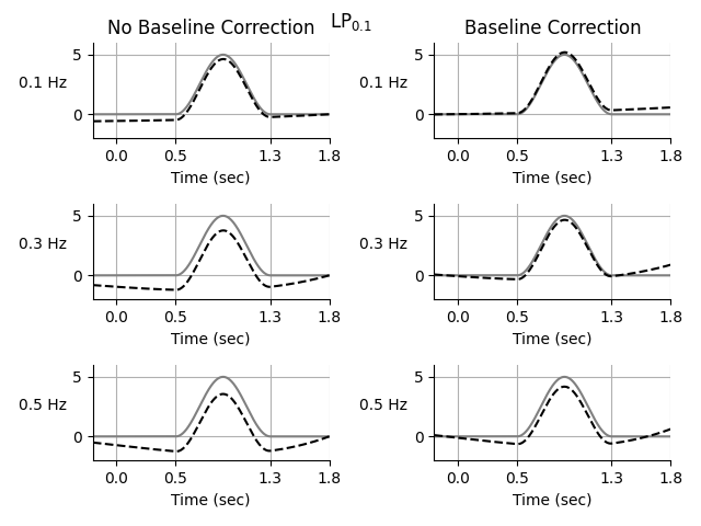
In an evolving discussion, Tanner et al. (2015) 8 suggest using baseline correction to remove slow drifts in data. However, Maess et al. (2016) 9 suggest that baseline correction, which is a form of high-passing, does not offer substantial advantages over standard high-pass filtering. Tanner et al. (2016) 10 rebutted that baseline correction can correct for problems with filtering.

To see what they mean, consider again our old simulated signal x from before:

def baseline_plot(x):
    all_axes = plt.subplots(3, 2)[1]
    for ri, (axes, freq) in enumerate(zip(all_axes, [0.1, 0.3, 0.5])):
        for ci, ax in enumerate(axes):
            if ci == 0:
                iir_hp = signal.iirfilter(4, freq / sfreq, btype='highpass',
                                          output='sos')
                x_hp = signal.sosfiltfilt(iir_hp, x, padlen=0)
            else:
                x_hp -= x_hp[t < 0].mean()
            ax.plot(t, x, color='0.5')
            ax.plot(t, x_hp, color='k', linestyle='--')
            if ri == 0:
                ax.set(title=('No ' if ci == 0 else '') +
                       'Baseline Correction')
            ax.set(xticks=tticks, ylim=ylim, xlim=xlim, xlabel=xlabel)
            ax.set_ylabel('%0.1f Hz' % freq, rotation=0,
                          horizontalalignment='right')
        mne.viz.adjust_axes(axes)
    mne.viz.tight_layout()
    plt.suptitle(title)
    plt.show()


baseline_plot(x)

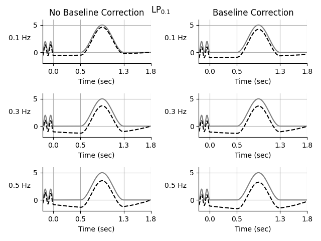
In response, Maess et al. (2016) 11 note that these simulations do not address cases of pre-stimulus activity that is shared across conditions, as applying baseline correction will effectively copy the topology outside the baseline period. We can see this if we give our signal x with some consistent pre-stimulus activity, which makes everything look bad.

Note

An important thing to keep in mind with these plots is that they are for a single simulated sensor. In multi-electrode recordings the topology (i.e., spatial pattern) of the pre-stimulus activity will leak into the post-stimulus period. This will likely create a spatially varying distortion of the time-domain signals, as the averaged pre-stimulus spatial pattern gets subtracted from the sensor time courses.

Putting some activity in the baseline period:

n_pre = (t < 0).sum()
sig_pre = 1 - np.cos(2 * np.pi * np.arange(n_pre) / (0.5 * n_pre))
x[:n_pre] += sig_pre
baseline_plot(x)

Both groups seem to acknowledge that the choices of filtering cutoffs, and perhaps even the application of baseline correction, depend on the characteristics of the data being investigated, especially when it comes to:

1. The frequency content of the underlying evoked activity relative to the filtering parameters.

2. The validity of the assumption of no consistent evoked activity in the baseline period.

We thus recommend carefully applying baseline correction and/or high-pass values based on the characteristics of the data to be analyzed.

Filtering defaults

Defaults in MNE-Python

Most often, filtering in MNE-Python is done at the mne.io.Raw level, and thus mne.io.Raw.filter() is used. This function under the hood (among other things) calls mne.filter.filter_data() to actually filter the data, which by default applies a zero-phase FIR filter designed using scipy.signal.firwin(). In Widmann et al. (2015) 7, they suggest a specific set of parameters to use for high-pass filtering, including:

“… providing a transition bandwidth of 25% of the lower passband edge but, where possible, not lower than 2 Hz and otherwise the distance from the passband edge to the critical frequency.”

In practice, this means that for each high-pass value l_freq or low-pass value h_freq below, you would get this corresponding l_trans_bandwidth or h_trans_bandwidth, respectively, if the sample rate were 100 Hz (i.e., Nyquist frequency of 50 Hz):

l_freq or h_freq	l_trans_bandwidth	h_trans_bandwidth
0.01	0.01	2.0
0.1	0.1	2.0
1.0	1.0	2.0
2.0	2.0	2.0
4.0	2.0	2.0
8.0	2.0	2.0
10.0	2.5	2.5
20.0	5.0	5.0
40.0	10.0	10.0
50.0	12.5	12.5

MNE-Python has adopted this definition for its high-pass (and low-pass) transition bandwidth choices when using l_trans_bandwidth='auto' and h_trans_bandwidth='auto'.

To choose the filter length automatically with filter_length='auto', the reciprocal of the shortest transition bandwidth is used to ensure decent attenuation at the stop frequency. Specifically, the reciprocal (in samples) is multiplied by 3.1, 3.3, or 5.0 for the Hann, Hamming, or Blackman windows, respectively, as selected by the fir_window argument for fir_design='firwin', and double these for fir_design='firwin2' mode.

Note

For fir_design='firwin2', the multiplicative factors are doubled compared to what is given in Ifeachor & Jervis (2002) 2 (p. 357), as scipy.signal.firwin2() has a smearing effect on the frequency response, which we compensate for by increasing the filter length. This is why fir_desgin='firwin' is preferred to fir_design='firwin2'.

In 0.14, we default to using a Hamming window in filter design, as it provides up to 53 dB of stop-band attenuation with small pass-band ripple.

Note

In band-pass applications, often a low-pass filter can operate effectively with fewer samples than the high-pass filter, so it is advisable to apply the high-pass and low-pass separately when using fir_design='firwin2'. For design mode fir_design='firwin', there is no need to separate the operations, as the lowpass and highpass elements are constructed separately to meet the transition band requirements.

For more information on how to use the MNE-Python filtering functions with real data, consult the preprocessing tutorial on Filtering and resampling data.

Defaults in MNE-C

MNE-C by default uses:

1. 5 Hz transition band for low-pass filters.

2. 3-sample transition band for high-pass filters.

3. Filter length of 8197 samples.

The filter is designed in the frequency domain, creating a linear-phase filter such that the delay is compensated for as is done with the MNE-Python phase='zero' filtering option.

Squared-cosine ramps are used in the transition regions. Because these are used in place of more gradual (e.g., linear) transitions, a given transition width will result in more temporal ringing but also more rapid attenuation than the same transition width in windowed FIR designs.

The default filter length will generally have excellent attenuation but long ringing for the sample rates typically encountered in M/EEG data (e.g. 500-2000 Hz).

Defaults in other software

A good but possibly outdated comparison of filtering in various software packages is available in Widmann et al. (2015) 7. Briefly:

• EEGLAB

  MNE-Python 0.14 defaults to behavior very similar to that of EEGLAB (see the EEGLAB filtering FAQ for more information).

• FieldTrip

  By default FieldTrip applies a forward-backward Butterworth IIR filter of order 4 (band-pass and band-stop filters) or 2 (for low-pass and high-pass filters). Similar filters can be achieved in MNE-Python when filtering with raw.filter(..., method='iir') (see also mne.filter.construct_iir_filter() for options). For more information, see e.g. the FieldTrip band-pass documentation.

Reporting Filters

On page 45 in Widmann et al. (2015) 7, there is a convenient list of important filter parameters that should be reported with each publication:

1. Filter type (high-pass, low-pass, band-pass, band-stop, FIR, IIR)

2. Cutoff frequency (including definition)

3. Filter order (or length)

4. Roll-off or transition bandwidth

5. Passband ripple and stopband attenuation

6. Filter delay (zero-phase, linear-phase, non-linear phase) and causality

7. Direction of computation (one-pass forward/reverse, or two-pass forward and reverse)

In the following, we will address how to deal with these parameters in MNE:

Filter type

Depending on the function or method used, the filter type can be specified. To name an example, in mne.filter.create_filter(), the relevant arguments would be l_freq, h_freq, method, and if the method is FIR fir_window and fir_design.

Cutoff frequency

The cutoff of FIR filters in MNE is defined as half-amplitude cutoff in the middle of the transition band. That is, if you construct a lowpass FIR filter with h_freq = 40, the filter function will provide a transition bandwidth that depends on the h_trans_bandwidth argument. The desired half-amplitude cutoff of the lowpass FIR filter is then at h_freq + transition_bandwidth/2..

Filter length (order) and transition bandwidth (roll-off)

In the Defaults in MNE-Python section, we have already talked about the default filter lengths and transition bandwidths that are used when no custom values are specified using the respective filter function’s arguments.

If you want to find out about the filter length and transition bandwidth that were used through the ‘auto’ setting, you can use mne.filter.create_filter() to print out the settings once more:

# Use the same settings as when calling e.g., `raw.filter()`
fir_coefs = mne.filter.create_filter(
    data=None,  # data is only used for sanity checking, not strictly needed
    sfreq=1000.,  # sfreq of your data in Hz
    l_freq=None,
    h_freq=40.,  # assuming a lowpass of 40 Hz
    method='fir',
    fir_window='hamming',
    fir_design='firwin',
    verbose=True)

# See the printed log for the transition bandwidth and filter length.
# Alternatively, get the filter length through:
filter_length = fir_coefs.shape[0]

Out:

No data specified. Sanity checks related to the length of the signal relative to the filter order will be skipped.
Setting up low-pass filter at 40 Hz

FIR filter parameters
---------------------
Designing a one-pass, zero-phase, non-causal lowpass filter:
- Windowed time-domain design (firwin) method
- Hamming window with 0.0194 passband ripple and 53 dB stopband attenuation
- Upper passband edge: 40.00 Hz
- Upper transition bandwidth: 10.00 Hz (-6 dB cutoff frequency: 45.00 Hz)
- Filter length: 331 samples (0.331 sec)

Note

If you are using an IIR filter, mne.filter.create_filter() will not print a filter length and transition bandwidth to the log. Instead, you can specify the roll-off with the iir_params argument or stay with the default, which is a fourth order (Butterworth) filter.

Passband ripple and stopband attenuation

When use standard scipy.signal.firwin() design (as for FIR filters in MNE), the passband ripple and stopband attenuation are dependent upon the window used in design. For standard windows the values are listed in this table (see Ifeachor & Jervis (2002) 2, p. 357):

Name of window function	Passband ripple	Stopband attenuation
Hann	0.0545 dB	44 dB
Hamming	0.0194 dB	53 dB
Blackman	0.0017 dB	74 dB

Filter delay and direction of computation

For reporting this information, it might be sufficient to read the docstring of the filter function or method that you apply. For example in the docstring of mne.filter.create_filter, for the phase parameter it says:

Phase of the filter, only used if method='fir'. By default, a symmetric linear-phase FIR filter is constructed. If phase='zero' (default), the delay of this filter is compensated for. If phase=='zero-double', then this filter is applied twice, once forward, and once backward. If ‘minimum’, then a minimum-phase, causal filter will be used.

Summary

When filtering, there are always trade-offs that should be considered. One important trade-off is between time-domain characteristics (like ringing) and frequency-domain attenuation characteristics (like effective transition bandwidth). Filters with sharp frequency cutoffs can produce outputs that ring for a long time when they operate on signals with frequency content in the transition band. In general, therefore, the wider a transition band that can be tolerated, the better behaved the filter will be in the time domain.

References

1(1,2)

Parks TW, Burrus CS (1987). Digital Filter Design. New York: Wiley-Interscience.

2(1,2,3,4)

Ifeachor, E. C., & Jervis, B. W. (2002). Digital Signal Processing: A Practical Approach. Prentice Hall.

3(1,2,3)

Vanrullen, R. (2011). Four common conceptual fallacies in mapping the time course of recognition. Perception Science, 2, 365.

4

Acunzo, D. J., MacKenzie, G., & van Rossum, M. C. W. (2012). Systematic biases in early ERP and ERF components as a result of high-pass filtering. Journal of Neuroscience Methods, 209(1), 212–218. https://doi.org/10.1016/j.jneumeth.2012.06.011

5

Rousselet, G. A. (2012). Does filtering preclude us from studying ERP time-courses? Frontiers in Psychology, 3(131)

6(1,2)

Widmann, A., & Schröger, E. (2012). Filter effects and filter artifacts in the analysis of electrophysiological data. Perception Science, 233.

7(1,2,3,4,5,6)

Widmann, A., Schröger, E., & Maess, B. (2015). Digital filter design for electrophysiological data – a practical approach. Journal of Neuroscience Methods, 250, 34–46. https://doi.org/10.1016/j.jneumeth.2014.08.002

8(1,2,3)

Tanner, D., Morgan-Short, K., & Luck, S. J. (2015). How inappropriate high-pass filters can produce artifactual effects and incorrect conclusions in ERP studies of language and cognition. Psychophysiology, 52(8), 997–1009. https://doi.org/10.1111/psyp.12437

9

Maess, B., Schröger, E., & Widmann, A. (2016). High-pass filters and baseline correction in M/EEG analysis. Commentary on: “How inappropriate high-pass filters can produce artifacts and incorrect conclusions in ERP studies of language and cognition.” Journal of Neuroscience Methods, 266, 164–165.

10

Tanner, D., Norton, J. J. S., Morgan-Short, K., & Luck, S. J. (2016). On high-pass filter artifacts (they’re real) and baseline correction (it’s a good idea) in ERP/ERMF analysis.

11

Maess, B., Schröger, E., & Widmann, A. (2016). High-pass filters and baseline correction in M/EEG analysis-continued discussion. Journal of Neuroscience Methods, 266, 171–172. Journal of Neuroscience Methods, 266, 166–170.

12

Kappenman E. & Luck, S. (2010). The effects of impedance on data quality and statistical significance in ERP recordings. Psychophysiology, 47, 888-904.

Estimated memory usage: 8 MB