Note
Click here to download the full example code
Brainstorm CTF phantom dataset tutorial
Here we compute the evoked from raw for the Brainstorm CTF phantom tutorial dataset. For comparison, see 1 and:
References
- 1
Tadel F, Baillet S, Mosher JC, Pantazis D, Leahy RM. Brainstorm: A User-Friendly Application for MEG/EEG Analysis. Computational Intelligence and Neuroscience, vol. 2011, Article ID 879716, 13 pages, 2011. doi:10.1155/2011/879716
# Authors: Eric Larson <larson.eric.d@gmail.com>
#
# License: BSD (3-clause)

import os.path as op
import numpy as np
import matplotlib.pyplot as plt

import mne
from mne import fit_dipole
from mne.datasets.brainstorm import bst_phantom_ctf
from mne.io import read_raw_ctf

print(__doc__)
The data were collected with a CTF system at 2400 Hz.
data_path = bst_phantom_ctf.data_path(verbose=True)

# Switch to these to use the higher-SNR data:
# raw_path = op.join(data_path, 'phantom_200uA_20150709_01.ds')
# dip_freq = 7.
raw_path = op.join(data_path, 'phantom_20uA_20150603_03.ds')
dip_freq = 23.
erm_path = op.join(data_path, 'emptyroom_20150709_01.ds')
raw = read_raw_ctf(raw_path, preload=True)
Out:
ds directory : /home/circleci/mne_data/MNE-brainstorm-data/bst_phantom_ctf/phantom_20uA_20150603_03.ds
    res4 data read.
    hc data read.
    Separate EEG position data file read.
    Quaternion matching (desired vs. transformed):
      -0.39   74.35    0.00 mm <->   -0.39   74.35   -0.00 mm (orig :  -39.23   63.82 -204.07 mm) diff =    0.000 mm
       0.39  -74.35    0.00 mm <->    0.39  -74.35   -0.00 mm (orig :   65.69  -41.53 -205.68 mm) diff =    0.000 mm
      75.00    0.00    0.00 mm <->   75.00   -0.00    0.00 mm (orig :   64.32   61.80 -226.08 mm) diff =    0.000 mm
    Coordinate transformations established.
    Polhemus data for 3 HPI coils added
    Device coordinate locations for 3 HPI coils added
    Measurement info composed.
Finding samples for /home/circleci/mne_data/MNE-brainstorm-data/bst_phantom_ctf/phantom_20uA_20150603_03.ds/phantom_20uA_20150603_03.meg4:
    System clock channel is available, checking which samples are valid.
    10 x 2400 = 24000 samples from 304 chs
Current compensation grade : 3
Reading 0 ... 23999  =      0.000 ...    10.000 secs...
The sinusoidal signal is generated on channel HDAC006, so we can use that to obtain precise timing.
sinusoid, times = raw[raw.ch_names.index('HDAC006-4408')]
plt.figure()
plt.plot(times[times < 1.], sinusoid.T[times < 1.])
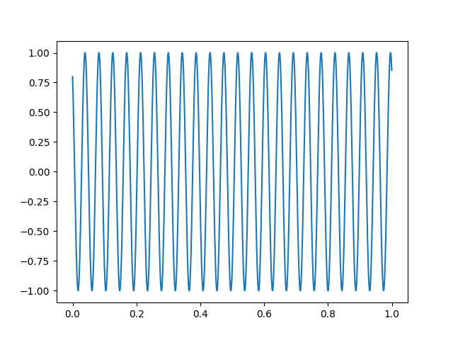
Let’s create some events using this signal by thresholding the sinusoid.
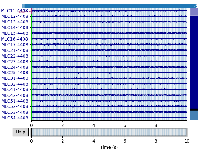
The CTF software compensation works reasonably well:
raw.plot()
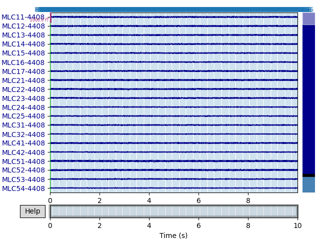
But here we can get slightly better noise suppression, lower localization bias, and a better dipole goodness of fit with spatio-temporal (tSSS) Maxwell filtering:
raw.apply_gradient_compensation(0)  # must un-do software compensation first
mf_kwargs = dict(origin=(0., 0., 0.), st_duration=10.)
raw = mne.preprocessing.maxwell_filter(raw, **mf_kwargs)
raw.plot()
Out:
Compensator constructed to change 3 -> 0
Applying compensator to loaded data
Maxwell filtering raw data
    No bad MEG channels
    Processing 0 gradiometers and 299 magnetometers (of which 290 are actually KIT gradiometers)
    Using origin 0.0, 0.0, 0.0 mm in the head frame
    Processing data using tSSS with st_duration=10.0
        Using 86/95 harmonic components for    0.000  (71/80 in, 15/15 out)
    Using loaded raw data
    Processing 1 data chunk
        Projecting  8 intersecting tSSS components for    0.000 -   10.000 sec (#1/1)
[done]
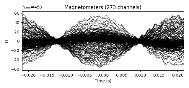
Our choice of tmin and tmax should capture exactly one cycle, so we can make the unusual choice of baselining using the entire epoch when creating our evoked data. We also then crop to a single time point (@t=0) because this is a peak in our signal.
tmin = -0.5 / dip_freq
tmax = -tmin
epochs = mne.Epochs(raw, events, event_id=1, tmin=tmin, tmax=tmax,
                    baseline=(None, None))
evoked = epochs.average()
evoked.plot(time_unit='s')
evoked.crop(0., 0.)
Out:
Not setting metadata
Not setting metadata
460 matching events found
Applying baseline correction (mode: mean)
0 projection items activated
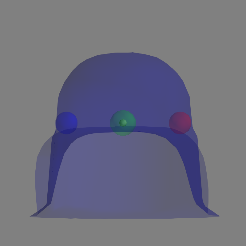
Let’s use a sphere head geometry model and let’s see the coordinate alignment and the sphere location.
sphere = mne.make_sphere_model(r0=(0., 0., 0.), head_radius=None)

mne.viz.plot_alignment(raw.info, subject='sample',
                       meg='helmet', bem=sphere, dig=True,
                       surfaces=['brain'])
del raw, epochs
Out:
Getting helmet for system CTF_275
To do a dipole fit, let’s use the covariance provided by the empty room recording.
raw_erm = read_raw_ctf(erm_path).apply_gradient_compensation(0)
raw_erm = mne.preprocessing.maxwell_filter(raw_erm, coord_frame='meg',
                                           **mf_kwargs)
cov = mne.compute_raw_covariance(raw_erm)
del raw_erm

dip, residual = fit_dipole(evoked, cov, sphere, verbose=True)
Out:
ds directory : /home/circleci/mne_data/MNE-brainstorm-data/bst_phantom_ctf/emptyroom_20150709_01.ds
    res4 data read.
    hc data read.
    Separate EEG position data file read.
    Quaternion matching (desired vs. transformed):
      -0.00   74.50    0.00 mm <->   -0.00   74.50   -0.00 mm (orig :  -50.17   57.61 -188.51 mm) diff =    0.000 mm
       0.00  -74.50    0.00 mm <->    0.00  -74.50    0.00 mm (orig :   60.49  -42.15 -190.81 mm) diff =    0.000 mm
      74.66    0.00    0.00 mm <->   74.66   -0.00    0.00 mm (orig :   53.03   61.29 -209.99 mm) diff =    0.000 mm
    Coordinate transformations established.
    Polhemus data for 3 HPI coils added
    Device coordinate locations for 3 HPI coils added
    Measurement info composed.
Finding samples for /home/circleci/mne_data/MNE-brainstorm-data/bst_phantom_ctf/emptyroom_20150709_01.ds/emptyroom_20150709_01.meg4:
    System clock channel is available, checking which samples are valid.
    100 x 600 = 60000 samples from 304 chs
Current compensation grade : 3
Compensator constructed to change 3 -> 0
Maxwell filtering raw data
    No bad MEG channels
    Processing 0 gradiometers and 299 magnetometers (of which 290 are actually KIT gradiometers)
    Using origin 0.0, 0.0, 0.0 mm in the meg frame (1.3, -8.8, -2.8 mm in the head frame)
    Processing data using tSSS with st_duration=10.0
        Using 90/95 harmonic components for    0.000  (75/80 in, 15/15 out)
    Loading raw data from disk
    Processing 10 data chunks
        Projecting  8 intersecting tSSS components for    0.000 -    9.998 sec  (#1/10)
        Projecting  8 intersecting tSSS components for   10.000 -   19.998 sec  (#2/10)
        Projecting  8 intersecting tSSS components for   20.000 -   29.998 sec  (#3/10)
        Projecting  8 intersecting tSSS components for   30.000 -   39.998 sec  (#4/10)
        Projecting  9 intersecting tSSS components for   40.000 -   49.998 sec  (#5/10)
        Projecting  8 intersecting tSSS components for   50.000 -   59.998 sec  (#6/10)
        Projecting  7 intersecting tSSS components for   60.000 -   69.998 sec  (#7/10)
        Projecting  9 intersecting tSSS components for   70.000 -   79.998 sec  (#8/10)
        Projecting  9 intersecting tSSS components for   80.000 -   89.998 sec  (#9/10)
        Projecting  8 intersecting tSSS components for   90.000 -   99.998 sec (#10/10)
[done]
Using up to 500 segments
Number of samples used : 60000
[done]
BEM               : <ConductorModel | Sphere (no layers): r0=[0.0, 0.0, 0.0] mm>
MRI transform     : identity
Sphere model      : origin at (   0.00    0.00    0.00) mm, max_rad =    0.1 mm
Guess grid        :   20.0 mm
Guess mindist     :    5.0 mm
Guess exclude     :   20.0 mm
Using standard MEG coil definitions.

Coordinate transformation: MRI (surface RAS) -> head
     1.000000  0.000000  0.000000       0.00 mm
     0.000000  1.000000  0.000000       0.00 mm
     0.000000  0.000000  1.000000       0.00 mm
     0.000000  0.000000  0.000000       1.00
Coordinate transformation: MEG device -> head
     0.999939 -0.002039 -0.010868      -2.00 mm
    -0.001115  0.959234 -0.282612     -20.74 mm
     0.011001  0.282607  0.959173       9.38 mm
     0.000000  0.000000  0.000000       1.00
0 bad channels total
Read 273 MEG channels from info
Read  26 MEG compensation channels from info
99 coil definitions read
Coordinate transformation: MEG device -> head
     0.999939 -0.002039 -0.010868      -2.00 mm
    -0.001115  0.959234 -0.282612     -20.74 mm
     0.011001  0.282607  0.959173       9.38 mm
     0.000000  0.000000  0.000000       1.00
5 compensation data sets in info
MEG coil definitions created in head coordinates.
Decomposing the sensor noise covariance matrix...
Removing 5 compensators from info because not all compensation channels were picked.
Computing rank from covariance with rank=None
    Using tolerance 1.9e-15 (2.2e-16 eps * 273 dim * 0.031  max singular value)
    Estimated rank (mag): 75
    MAG: rank 75 computed from 273 data channels with 0 projectors
    Setting small MAG eigenvalues to zero (without PCA)
    Created the whitener using a noise covariance matrix with rank 75 (198 small eigenvalues omitted)

---- Computing the forward solution for the guesses...
Making a spherical guess space with radius    98.6 mm...
Filtering (grid =     20 mm)...
Surface CM = (   0.0    0.0    0.0) mm
Surface fits inside a sphere with radius   98.6 mm
Surface extent:
    x =  -98.6 ...   98.6 mm
    y =  -98.6 ...   98.6 mm
    z =  -98.6 ...   98.6 mm
Grid extent:
    x = -100.0 ...  100.0 mm
    y = -100.0 ...  100.0 mm
    z = -100.0 ...  100.0 mm
1331 sources before omitting any.
484 sources after omitting infeasible sources not within 20.0 - 98.6 mm.
436 sources remaining after excluding the sources outside the surface and less than    5.0 mm inside.
Go through all guess source locations...
[done 436 sources]
---- Fitted :     0.0 ms
No projector specified for this dataset. Please consider the method self.add_proj.
1 time points fitted
Compare the actual position with the estimated one.
expected_pos = np.array([18., 0., 49.])
diff = np.sqrt(np.sum((dip.pos[0] * 1000 - expected_pos) ** 2))
print('Actual pos:     %s mm' % np.array_str(expected_pos, precision=1))
print('Estimated pos:  %s mm' % np.array_str(dip.pos[0] * 1000, precision=1))
print('Difference:     %0.1f mm' % diff)
print('Amplitude:      %0.1f nAm' % (1e9 * dip.amplitude[0]))
print('GOF:            %0.1f %%' % dip.gof[0])
Out:
Actual pos:     [18.  0. 49.] mm
Estimated pos:  [18.5 -2.2 44.6] mm
Difference:     4.9 mm
Amplitude:      10.0 nAm
GOF:            96.5 %
Total running time of the script: ( 0 minutes 25.776 seconds)
Estimated memory usage: 557 MB