Note
Click here to download the full example code
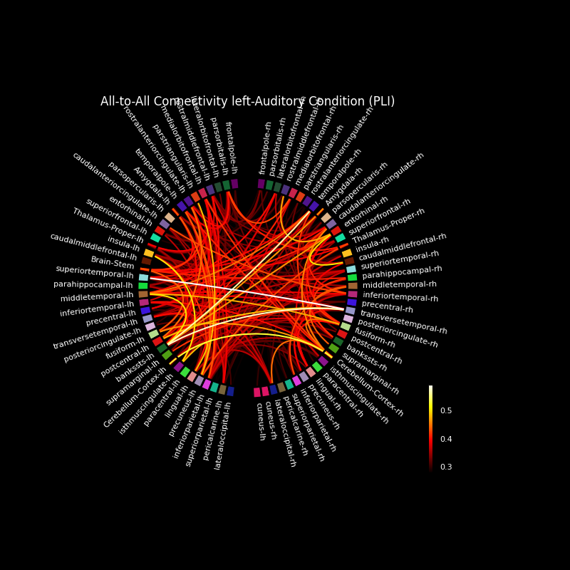
Compute mixed source space connectivity and visualize it using a circular graph
This example computes the all-to-all connectivity between 75 regions in a mixed source space based on dSPM inverse solutions and a FreeSurfer cortical parcellation. The connectivity is visualized using a circular graph which is ordered based on the locations of the regions in the axial plane.
# Author: Annalisa Pascarella <a.pascarella@iac.cnr.it>
#
# License: BSD (3-clause)

import os.path as op
import numpy as np
import mne
import matplotlib.pyplot as plt

from mne.datasets import sample
from mne import setup_volume_source_space, setup_source_space
from mne import make_forward_solution
from mne.io import read_raw_fif
from mne.minimum_norm import make_inverse_operator, apply_inverse_epochs
from mne.connectivity import spectral_connectivity
from mne.viz import circular_layout, plot_connectivity_circle

# Set directories
data_path = sample.data_path()
subject = 'sample'
data_dir = op.join(data_path, 'MEG', subject)
subjects_dir = op.join(data_path, 'subjects')
bem_dir = op.join(subjects_dir, subject, 'bem')

# Set file names
fname_aseg = op.join(subjects_dir, subject, 'mri', 'aseg.mgz')

fname_model = op.join(bem_dir, '%s-5120-bem.fif' % subject)
fname_bem = op.join(bem_dir, '%s-5120-bem-sol.fif' % subject)

fname_raw = data_dir + '/sample_audvis_filt-0-40_raw.fif'
fname_trans = data_dir + '/sample_audvis_raw-trans.fif'
fname_cov = data_dir + '/ernoise-cov.fif'
fname_event = data_dir + '/sample_audvis_filt-0-40_raw-eve.fif'

# List of sub structures we are interested in. We select only the
# sub structures we want to include in the source space
labels_vol = ['Left-Amygdala',
              'Left-Thalamus-Proper',
              'Left-Cerebellum-Cortex',
              'Brain-Stem',
              'Right-Amygdala',
              'Right-Thalamus-Proper',
              'Right-Cerebellum-Cortex']

# Setup a surface-based source space, oct5 is not very dense (just used
# to speed up this example; we recommend oct6 in actual analyses)
src = setup_source_space(subject, subjects_dir=subjects_dir,
                         spacing='oct5', add_dist=False)

# Setup a volume source space
# set pos=10.0 for speed, not very accurate; we recommend something smaller
# like 5.0 in actual analyses:
vol_src = setup_volume_source_space(
    subject, mri=fname_aseg, pos=10.0, bem=fname_model,
    add_interpolator=False,  # just for speed, usually use True
    volume_label=labels_vol, subjects_dir=subjects_dir)
# Generate the mixed source space
src += vol_src

# Load data
raw = read_raw_fif(fname_raw)
raw.pick_types(meg=True, eeg=False, eog=True, stim=True).load_data()
events = mne.find_events(raw)
noise_cov = mne.read_cov(fname_cov)

# compute the fwd matrix
fwd = make_forward_solution(raw.info, fname_trans, src, fname_bem,
                            mindist=5.0)  # ignore sources<=5mm from innerskull
del src

# Define epochs for left-auditory condition
event_id, tmin, tmax = 1, -0.2, 0.5
reject = dict(mag=4e-12, grad=4000e-13, eog=150e-6)
epochs = mne.Epochs(raw, events, event_id, tmin, tmax,
                    reject=reject, preload=False)
del raw

# Compute inverse solution and for each epoch
snr = 1.0           # use smaller SNR for raw data
inv_method = 'dSPM'
parc = 'aparc'      # the parcellation to use, e.g., 'aparc' 'aparc.a2009s'

lambda2 = 1.0 / snr ** 2

# Compute inverse operator
inverse_operator = make_inverse_operator(
    epochs.info, fwd, noise_cov, depth=None, fixed=False)
del fwd

stcs = apply_inverse_epochs(epochs, inverse_operator, lambda2, inv_method,
                            pick_ori=None, return_generator=True)

# Get labels for FreeSurfer 'aparc' cortical parcellation with 34 labels/hemi
labels_parc = mne.read_labels_from_annot(subject, parc=parc,
                                         subjects_dir=subjects_dir)

# Average the source estimates within each label of the cortical parcellation
# and each sub structures contained in the src space
# If mode = 'mean_flip' this option is used only for the cortical label
src = inverse_operator['src']
label_ts = mne.extract_label_time_course(
    stcs, labels_parc, src, mode='mean_flip', allow_empty=True,
    return_generator=True)

# We compute the connectivity in the alpha band and plot it using a circular
# graph layout
fmin = 8.
fmax = 13.
sfreq = epochs.info['sfreq']  # the sampling frequency
con, freqs, times, n_epochs, n_tapers = spectral_connectivity(
    label_ts, method='pli', mode='multitaper', sfreq=sfreq, fmin=fmin,
    fmax=fmax, faverage=True, mt_adaptive=True, n_jobs=1)

# We create a list of Label containing also the sub structures
labels_aseg = mne.get_volume_labels_from_src(src, subject, subjects_dir)
labels = labels_parc + labels_aseg

# read colors
node_colors = [label.color for label in labels]

# We reorder the labels based on their location in the left hemi
label_names = [label.name for label in labels]
lh_labels = [name for name in label_names if name.endswith('lh')]
rh_labels = [name for name in label_names if name.endswith('rh')]

# Get the y-location of the label
label_ypos_lh = list()
for name in lh_labels:
    idx = label_names.index(name)
    ypos = np.mean(labels[idx].pos[:, 1])
    label_ypos_lh.append(ypos)
try:
    idx = label_names.index('Brain-Stem')
except ValueError:
    pass
else:
    ypos = np.mean(labels[idx].pos[:, 1])
    lh_labels.append('Brain-Stem')
    label_ypos_lh.append(ypos)


# Reorder the labels based on their location
lh_labels = [label for (yp, label) in sorted(zip(label_ypos_lh, lh_labels))]

# For the right hemi
rh_labels = [label[:-2] + 'rh' for label in lh_labels
             if label != 'Brain-Stem' and label[:-2] + 'rh' in rh_labels]

# Save the plot order
node_order = lh_labels[::-1] + rh_labels

node_angles = circular_layout(label_names, node_order, start_pos=90,
                              group_boundaries=[0, len(label_names) // 2])


# Plot the graph using node colors from the FreeSurfer parcellation. We only
# show the 300 strongest connections.
conmat = con[:, :, 0]
fig = plt.figure(num=None, figsize=(8, 8), facecolor='black')
plot_connectivity_circle(conmat, label_names, n_lines=300,
                         node_angles=node_angles, node_colors=node_colors,
                         title='All-to-All Connectivity left-Auditory '
                         'Condition (PLI)', fig=fig)
Out:
Setting up the source space with the following parameters:

SUBJECTS_DIR = /home/circleci/mne_data/MNE-sample-data/subjects
Subject      = sample
Surface      = white
Octahedron subdivision grade 5

>>> 1. Creating the source space...

Doing the octahedral vertex picking...
Loading /home/circleci/mne_data/MNE-sample-data/subjects/sample/surf/lh.white...
Mapping lh sample -> oct (5) ...
    Triangle neighbors and vertex normals...
Loading geometry from /home/circleci/mne_data/MNE-sample-data/subjects/sample/surf/lh.sphere...
Setting up the triangulation for the decimated surface...
loaded lh.white 1026/155407 selected to source space (oct = 5)

Loading /home/circleci/mne_data/MNE-sample-data/subjects/sample/surf/rh.white...
Mapping rh sample -> oct (5) ...
    Triangle neighbors and vertex normals...
Loading geometry from /home/circleci/mne_data/MNE-sample-data/subjects/sample/surf/rh.sphere...
Setting up the triangulation for the decimated surface...
loaded rh.white 1026/156866 selected to source space (oct = 5)

You are now one step closer to computing the gain matrix
BEM              : /home/circleci/mne_data/MNE-sample-data/subjects/sample/bem/sample-5120-bem.fif
grid                  : 10.0 mm
mindist               : 5.0 mm
MRI volume            : /home/circleci/mne_data/MNE-sample-data/subjects/sample/mri/aseg.mgz

Reading /home/circleci/mne_data/MNE-sample-data/subjects/sample/mri/aseg.mgz...

Loaded inner skull from /home/circleci/mne_data/MNE-sample-data/subjects/sample/bem/sample-5120-bem.fif (2562 nodes)
Surface CM = (   0.7  -10.0   44.3) mm
Surface fits inside a sphere with radius   91.8 mm
Surface extent:
    x =  -66.7 ...   68.8 mm
    y =  -88.0 ...   79.0 mm
    z =  -44.5 ...  105.8 mm
Grid extent:
    x =  -70.0 ...   70.0 mm
    y =  -90.0 ...   80.0 mm
    z =  -50.0 ...  110.0 mm
4590 sources before omitting any.
2961 sources after omitting infeasible sources not within 0.0 - 91.8 mm.
Source spaces are in MRI coordinates.
Checking that the sources are inside the surface and at least    5.0 mm away (will take a few...)
    Skipping interior check for 346 sources that fit inside a sphere of radius   43.6 mm
    Skipping solid angle check for 1275 points using Qhull
    1372 source space points omitted because they are outside the inner skull surface.
    283 source space points omitted because of the    5.0-mm distance limit.
1306 sources remaining after excluding the sources outside the surface and less than    5.0 mm inside.
    Selected 2 voxels from Left-Amygdala
    Selected 9 voxels from Left-Thalamus-Proper
    Selected 33 voxels from Left-Cerebellum-Cortex
    Selected 21 voxels from Brain-Stem
    Selected 1 voxel from Right-Amygdala
    Selected 7 voxels from Right-Thalamus-Proper
    Selected 44 voxels from Right-Cerebellum-Cortex
Adjusting the neighborhood info.
Source space : MRI voxel -> MRI (surface RAS)
     0.010000  0.000000  0.000000     -70.00 mm
     0.000000  0.010000  0.000000     -90.00 mm
     0.000000  0.000000  0.010000     -50.00 mm
     0.000000  0.000000  0.000000       1.00
MRI volume : MRI voxel -> MRI (surface RAS)
    -0.001000  0.000000  0.000000     128.00 mm
     0.000000  0.000000  0.001000    -128.00 mm
     0.000000 -0.001000  0.000000     128.00 mm
     0.000000  0.000000  0.000000       1.00
MRI volume : MRI (surface RAS) -> RAS (non-zero origin)
     1.000000 -0.000000 -0.000000      -5.27 mm
    -0.000000  1.000000 -0.000000       9.04 mm
    -0.000000  0.000000  1.000000     -27.29 mm
     0.000000  0.000000  0.000000       1.00
Opening raw data file /home/circleci/mne_data/MNE-sample-data/MEG/sample/sample_audvis_filt-0-40_raw.fif...
    Read a total of 4 projection items:
        PCA-v1 (1 x 10²)  idle
        PCA-v2 (1 x 10²)  idle
        PCA-v3 (1 x 10²)  idle
        Average EEG reference (1 x 60)  idle
    Range : 6450 ... 48149 =     42.956 ...   320.665 secs
Ready.
Removing projector <Projection | Average EEG reference, active : False, n_channels : 60>
Reading 0 ... 41699  =      0.000 ...   277.709 secs...
319 events found
Event IDs: [ 1  2  3  4  5 32]
    306 x 306 full covariance (kind = 1) found.
    Read a total of 3 projection items:
        PCA-v1 (1 x 10²) active
        PCA-v2 (1 x 10²) active
        PCA-v3 (1 x 10²) active
Source space          : <SourceSpaces: [<surface (lh), n_vertices=155407, n_used=1026>, <surface (rh), n_vertices=156866, n_used=1026>, <volume (Left-Amygdala), n_used=2>, <volume (Left-Thalamus-Proper), n_used=9>, <volume (Left-Cerebellum-Cortex), n_used=33>, <volume (Brain-Stem), n_used=21>, <volume (Right-Amygdala), n_used=1>, <volume (Right-Thalamus-Proper), n_used=7>, <volume (Right-Cerebellum-Cortex), n_used=44>] MRI (surface RAS) coords, subject 'sample', ~30.5 MB>
MRI -> head transform : /home/circleci/mne_data/MNE-sample-data/MEG/sample/sample_audvis_raw-trans.fif
Measurement data      : instance of Info
Conductor model   : /home/circleci/mne_data/MNE-sample-data/subjects/sample/bem/sample-5120-bem-sol.fif
Accurate field computations
Do computations in head coordinates
Free source orientations

Read 9 source spaces a total of 2169 active source locations

Coordinate transformation: MRI (surface RAS) -> head
     0.999310  0.009985 -0.035787      -3.17 mm
     0.012759  0.812405  0.582954       6.86 mm
     0.034894 -0.583008  0.811716      28.88 mm
     0.000000  0.000000  0.000000       1.00

Read 305 MEG channels from info
99 coil definitions read
Coordinate transformation: MEG device -> head
     0.991420 -0.039936 -0.124467      -6.13 mm
     0.060661  0.984012  0.167456       0.06 mm
     0.115790 -0.173570  0.977991      64.74 mm
     0.000000  0.000000  0.000000       1.00
MEG coil definitions created in head coordinates.
Source spaces are now in head coordinates.

Setting up the BEM model using /home/circleci/mne_data/MNE-sample-data/subjects/sample/bem/sample-5120-bem-sol.fif...

Loading surfaces...

Loading the solution matrix...

Homogeneous model surface loaded.
Loaded linear_collocation BEM solution from /home/circleci/mne_data/MNE-sample-data/subjects/sample/bem/sample-5120-bem-sol.fif
Employing the head->MRI coordinate transform with the BEM model.
BEM model sample-5120-bem-sol.fif is now set up

Source spaces are in head coordinates.
Checking that the sources are inside the surface and at least    5.0 mm away (will take a few...)
    Skipping interior check for 211 sources that fit inside a sphere of radius   43.6 mm
    Skipping solid angle check for 0 points using Qhull
    84 source space point omitted because of the    5.0-mm distance limit.
    Skipping interior check for 219 sources that fit inside a sphere of radius   43.6 mm
    Skipping solid angle check for 0 points using Qhull
    84 source space point omitted because of the    5.0-mm distance limit.
    Skipping interior check for 2 sources that fit inside a sphere of radius   43.6 mm
    Skipping solid angle check for 0 points using Qhull
    Skipping interior check for 9 sources that fit inside a sphere of radius   43.6 mm
    Skipping solid angle check for 0 points using Qhull
    Skipping interior check for 1 sources that fit inside a sphere of radius   43.6 mm
    Skipping solid angle check for 0 points using Qhull
    Skipping interior check for 8 sources that fit inside a sphere of radius   43.6 mm
    Skipping solid angle check for 0 points using Qhull
    Skipping interior check for 1 sources that fit inside a sphere of radius   43.6 mm
    Skipping solid angle check for 0 points using Qhull
    Skipping interior check for 7 sources that fit inside a sphere of radius   43.6 mm
    Skipping solid angle check for 0 points using Qhull
    Skipping interior check for 1 sources that fit inside a sphere of radius   43.6 mm
    Skipping solid angle check for 0 points using Qhull

Setting up compensation data...
    No compensation set. Nothing more to do.

Composing the field computation matrix...
Computing MEG at 2001 source locations (free orientations)...

Finished.
Not setting metadata
Not setting metadata
72 matching events found
Setting baseline interval to [-0.19979521315838786, 0.0] sec
Applying baseline correction (mode: mean)
Created an SSP operator (subspace dimension = 3)
3 projection items activated
info["bads"] and noise_cov["bads"] do not match, excluding bad channels from both
Computing inverse operator with 305 channels.
    305 out of 305 channels remain after picking
Selected 305 channels
Whitening the forward solution.
    Created an SSP operator (subspace dimension = 3)
Computing rank from covariance with rank=None
    Using tolerance 1.3e-13 (2.2e-16 eps * 305 dim * 2  max singular value)
    Estimated rank (mag + grad): 302
    MEG: rank 302 computed from 305 data channels with 3 projectors
    Setting small MEG eigenvalues to zero (without PCA)
Creating the source covariance matrix
Adjusting source covariance matrix.
Computing SVD of whitened and weighted lead field matrix.
    largest singular value = 6.38137
    scaling factor to adjust the trace = 1.17172e+21
Reading labels from parcellation...
   read 34 labels from /home/circleci/mne_data/MNE-sample-data/subjects/sample/label/lh.aparc.annot
   read 34 labels from /home/circleci/mne_data/MNE-sample-data/subjects/sample/label/rh.aparc.annot
Connectivity computation...
Preparing the inverse operator for use...
    Scaled noise and source covariance from nave = 1 to nave = 1
    Created the regularized inverter
    Created an SSP operator (subspace dimension = 3)
    Created the whitener using a noise covariance matrix with rank 302 (3 small eigenvalues omitted)
    Computing noise-normalization factors (dSPM)...
[done]
Picked 305 channels from the data
Computing inverse...
    Eigenleads need to be weighted ...
Processing epoch : 1 / 72 (at most)
combining the current components...
Extracting time courses for 75 labels (mode: mean_flip)
only using indices for lower-triangular matrix
    computing connectivity for 2775 connections
    using t=0.000s..0.699s for estimation (106 points)
    frequencies: 8.5Hz..12.7Hz (4 points)
    connectivity scores will be averaged for each band
    Using multitaper spectrum estimation with 7 DPSS windows
    the following metrics will be computed: PLI
    computing connectivity for epoch 1
Processing epoch : 2 / 72 (at most)
combining the current components...
Extracting time courses for 75 labels (mode: mean_flip)
    computing connectivity for epoch 2
Processing epoch : 3 / 72 (at most)
combining the current components...
Extracting time courses for 75 labels (mode: mean_flip)
    computing connectivity for epoch 3
Processing epoch : 4 / 72 (at most)
combining the current components...
Extracting time courses for 75 labels (mode: mean_flip)
    computing connectivity for epoch 4
Processing epoch : 5 / 72 (at most)
combining the current components...
Extracting time courses for 75 labels (mode: mean_flip)
    computing connectivity for epoch 5
Processing epoch : 6 / 72 (at most)
combining the current components...
Extracting time courses for 75 labels (mode: mean_flip)
    computing connectivity for epoch 6
Processing epoch : 7 / 72 (at most)
combining the current components...
Extracting time courses for 75 labels (mode: mean_flip)
    computing connectivity for epoch 7
Processing epoch : 8 / 72 (at most)
combining the current components...
Extracting time courses for 75 labels (mode: mean_flip)
    computing connectivity for epoch 8
Processing epoch : 9 / 72 (at most)
combining the current components...
Extracting time courses for 75 labels (mode: mean_flip)
    computing connectivity for epoch 9
Processing epoch : 10 / 72 (at most)
combining the current components...
Extracting time courses for 75 labels (mode: mean_flip)
    computing connectivity for epoch 10
    Rejecting  epoch based on EOG : ['EOG 061']
Processing epoch : 11 / 72 (at most)
combining the current components...
Extracting time courses for 75 labels (mode: mean_flip)
    computing connectivity for epoch 11
Processing epoch : 12 / 72 (at most)
combining the current components...
Extracting time courses for 75 labels (mode: mean_flip)
    computing connectivity for epoch 12
Processing epoch : 13 / 72 (at most)
combining the current components...
Extracting time courses for 75 labels (mode: mean_flip)
    computing connectivity for epoch 13
    Rejecting  epoch based on EOG : ['EOG 061']
    Rejecting  epoch based on EOG : ['EOG 061']
Processing epoch : 14 / 72 (at most)
combining the current components...
Extracting time courses for 75 labels (mode: mean_flip)
    computing connectivity for epoch 14
Processing epoch : 15 / 72 (at most)
combining the current components...
Extracting time courses for 75 labels (mode: mean_flip)
    computing connectivity for epoch 15
Processing epoch : 16 / 72 (at most)
combining the current components...
Extracting time courses for 75 labels (mode: mean_flip)
    computing connectivity for epoch 16
Processing epoch : 17 / 72 (at most)
combining the current components...
Extracting time courses for 75 labels (mode: mean_flip)
    computing connectivity for epoch 17
    Rejecting  epoch based on EOG : ['EOG 061']
Processing epoch : 18 / 72 (at most)
combining the current components...
Extracting time courses for 75 labels (mode: mean_flip)
    computing connectivity for epoch 18
Processing epoch : 19 / 72 (at most)
combining the current components...
Extracting time courses for 75 labels (mode: mean_flip)
    computing connectivity for epoch 19
Processing epoch : 20 / 72 (at most)
combining the current components...
Extracting time courses for 75 labels (mode: mean_flip)
    computing connectivity for epoch 20
    Rejecting  epoch based on EOG : ['EOG 061']
Processing epoch : 21 / 72 (at most)
combining the current components...
Extracting time courses for 75 labels (mode: mean_flip)
    computing connectivity for epoch 21
Processing epoch : 22 / 72 (at most)
combining the current components...
Extracting time courses for 75 labels (mode: mean_flip)
    computing connectivity for epoch 22
Processing epoch : 23 / 72 (at most)
combining the current components...
Extracting time courses for 75 labels (mode: mean_flip)
    computing connectivity for epoch 23
    Rejecting  epoch based on MAG : ['MEG 1711']
Processing epoch : 24 / 72 (at most)
combining the current components...
Extracting time courses for 75 labels (mode: mean_flip)
    computing connectivity for epoch 24
Processing epoch : 25 / 72 (at most)
combining the current components...
Extracting time courses for 75 labels (mode: mean_flip)
    computing connectivity for epoch 25
Processing epoch : 26 / 72 (at most)
combining the current components...
Extracting time courses for 75 labels (mode: mean_flip)
    computing connectivity for epoch 26
Processing epoch : 27 / 72 (at most)
combining the current components...
Extracting time courses for 75 labels (mode: mean_flip)
    computing connectivity for epoch 27
Processing epoch : 28 / 72 (at most)
combining the current components...
Extracting time courses for 75 labels (mode: mean_flip)
    computing connectivity for epoch 28
    Rejecting  epoch based on EOG : ['EOG 061']
Processing epoch : 29 / 72 (at most)
combining the current components...
Extracting time courses for 75 labels (mode: mean_flip)
    computing connectivity for epoch 29
Processing epoch : 30 / 72 (at most)
combining the current components...
Extracting time courses for 75 labels (mode: mean_flip)
    computing connectivity for epoch 30
Processing epoch : 31 / 72 (at most)
combining the current components...
Extracting time courses for 75 labels (mode: mean_flip)
    computing connectivity for epoch 31
    Rejecting  epoch based on EOG : ['EOG 061']
Processing epoch : 32 / 72 (at most)
combining the current components...
Extracting time courses for 75 labels (mode: mean_flip)
    computing connectivity for epoch 32
Processing epoch : 33 / 72 (at most)
combining the current components...
Extracting time courses for 75 labels (mode: mean_flip)
    computing connectivity for epoch 33
    Rejecting  epoch based on EOG : ['EOG 061']
Processing epoch : 34 / 72 (at most)
combining the current components...
Extracting time courses for 75 labels (mode: mean_flip)
    computing connectivity for epoch 34
Processing epoch : 35 / 72 (at most)
combining the current components...
Extracting time courses for 75 labels (mode: mean_flip)
    computing connectivity for epoch 35
    Rejecting  epoch based on EOG : ['EOG 061']
    Rejecting  epoch based on EOG : ['EOG 061']
Processing epoch : 36 / 72 (at most)
combining the current components...
Extracting time courses for 75 labels (mode: mean_flip)
    computing connectivity for epoch 36
    Rejecting  epoch based on EOG : ['EOG 061']
    Rejecting  epoch based on EOG : ['EOG 061']
Processing epoch : 37 / 72 (at most)
combining the current components...
Extracting time courses for 75 labels (mode: mean_flip)
    computing connectivity for epoch 37
Processing epoch : 38 / 72 (at most)
combining the current components...
Extracting time courses for 75 labels (mode: mean_flip)
    computing connectivity for epoch 38
Processing epoch : 39 / 72 (at most)
combining the current components...
Extracting time courses for 75 labels (mode: mean_flip)
    computing connectivity for epoch 39
Processing epoch : 40 / 72 (at most)
combining the current components...
Extracting time courses for 75 labels (mode: mean_flip)
    computing connectivity for epoch 40
Processing epoch : 41 / 72 (at most)
combining the current components...
Extracting time courses for 75 labels (mode: mean_flip)
    computing connectivity for epoch 41
Processing epoch : 42 / 72 (at most)
combining the current components...
Extracting time courses for 75 labels (mode: mean_flip)
    computing connectivity for epoch 42
Processing epoch : 43 / 72 (at most)
combining the current components...
Extracting time courses for 75 labels (mode: mean_flip)
    computing connectivity for epoch 43
Processing epoch : 44 / 72 (at most)
combining the current components...
Extracting time courses for 75 labels (mode: mean_flip)
    computing connectivity for epoch 44
    Rejecting  epoch based on EOG : ['EOG 061']
Processing epoch : 45 / 72 (at most)
combining the current components...
Extracting time courses for 75 labels (mode: mean_flip)
    computing connectivity for epoch 45
    Rejecting  epoch based on EOG : ['EOG 061']
Processing epoch : 46 / 72 (at most)
combining the current components...
Extracting time courses for 75 labels (mode: mean_flip)
    computing connectivity for epoch 46
Processing epoch : 47 / 72 (at most)
combining the current components...
Extracting time courses for 75 labels (mode: mean_flip)
    computing connectivity for epoch 47
Processing epoch : 48 / 72 (at most)
combining the current components...
Extracting time courses for 75 labels (mode: mean_flip)
    computing connectivity for epoch 48
    Rejecting  epoch based on EOG : ['EOG 061']
    Rejecting  epoch based on EOG : ['EOG 061']
Processing epoch : 49 / 72 (at most)
combining the current components...
Extracting time courses for 75 labels (mode: mean_flip)
    computing connectivity for epoch 49
Processing epoch : 50 / 72 (at most)
combining the current components...
Extracting time courses for 75 labels (mode: mean_flip)
    computing connectivity for epoch 50
Processing epoch : 51 / 72 (at most)
combining the current components...
Extracting time courses for 75 labels (mode: mean_flip)
    computing connectivity for epoch 51
Processing epoch : 52 / 72 (at most)
combining the current components...
Extracting time courses for 75 labels (mode: mean_flip)
    computing connectivity for epoch 52
Processing epoch : 53 / 72 (at most)
combining the current components...
Extracting time courses for 75 labels (mode: mean_flip)
    computing connectivity for epoch 53
Processing epoch : 54 / 72 (at most)
combining the current components...
Extracting time courses for 75 labels (mode: mean_flip)
    computing connectivity for epoch 54
Processing epoch : 55 / 72 (at most)
combining the current components...
Extracting time courses for 75 labels (mode: mean_flip)
    computing connectivity for epoch 55
[done]
    assembling connectivity matrix (filling the upper triangular region of the matrix)
[Connectivity computation done]
Save the figure (optional)
By default matplotlib does not save using the facecolor, even though this was set when the figure was generated. If not set via savefig, the labels, title, and legend will be cut off from the output png file:
>>> fname_fig = data_path + '/MEG/sample/plot_mixed_connect.png'
>>> plt.savefig(fname_fig, facecolor='black')
Total running time of the script: ( 0 minutes 15.725 seconds)
Estimated memory usage: 134 MB