Note
Click here to download the full example code
Compute sparse inverse solution with mixed norm: MxNE and irMxNE
Runs an (ir)MxNE (L1/L2 1 or L0.5/L2 2 mixed norm) inverse solver. L0.5/L2 is done with irMxNE which allows for sparser source estimates with less amplitude bias due to the non-convexity of the L0.5/L2 mixed norm penalty.
# Author: Alexandre Gramfort <alexandre.gramfort@inria.fr>
#         Daniel Strohmeier <daniel.strohmeier@tu-ilmenau.de>
#
# License: BSD (3-clause)


import numpy as np

import mne
from mne.datasets import sample
from mne.inverse_sparse import mixed_norm, make_stc_from_dipoles
from mne.minimum_norm import make_inverse_operator, apply_inverse
from mne.viz import (plot_sparse_source_estimates,
                     plot_dipole_locations, plot_dipole_amplitudes)

print(__doc__)

data_path = sample.data_path()
fwd_fname = data_path + '/MEG/sample/sample_audvis-meg-eeg-oct-6-fwd.fif'
ave_fname = data_path + '/MEG/sample/sample_audvis-ave.fif'
cov_fname = data_path + '/MEG/sample/sample_audvis-shrunk-cov.fif'
subjects_dir = data_path + '/subjects'

# Read noise covariance matrix
cov = mne.read_cov(cov_fname)
# Handling average file
condition = 'Left Auditory'
evoked = mne.read_evokeds(ave_fname, condition=condition, baseline=(None, 0))
evoked.crop(tmin=0, tmax=0.3)
# Handling forward solution
forward = mne.read_forward_solution(fwd_fname)
Out:
    365 x 365 full covariance (kind = 1) found.
    Read a total of 4 projection items:
        PCA-v1 (1 x 10²) active
        PCA-v2 (1 x 10²) active
        PCA-v3 (1 x 10²) active
        Average EEG reference (1 x 59) active
Reading /home/circleci/mne_data/MNE-sample-data/MEG/sample/sample_audvis-ave.fif ...
    Read a total of 4 projection items:
        PCA-v1 (1 x 10²) active
        PCA-v2 (1 x 10²) active
        PCA-v3 (1 x 10²) active
        Average EEG reference (1 x 60) active
    Found the data of interest:
        t =    -199.80 ...     499.49 ms (Left Auditory)
        0 CTF compensation matrices available
        nave = 55 - aspect type = 100
Projections have already been applied. Setting proj attribute to True.
Applying baseline correction (mode: mean)
Reading forward solution from /home/circleci/mne_data/MNE-sample-data/MEG/sample/sample_audvis-meg-eeg-oct-6-fwd.fif...
    Reading a source space...
    Computing patch statistics...
    Patch information added...
    Distance information added...
    [done]
    Reading a source space...
    Computing patch statistics...
    Patch information added...
    Distance information added...
    [done]
    2 source spaces read
    Desired named matrix (kind = 3523) not available
    Read MEG forward solution (7498 sources, 306 channels, free orientations)
    Desired named matrix (kind = 3523) not available
    Read EEG forward solution (7498 sources, 60 channels, free orientations)
    MEG and EEG forward solutions combined
    Source spaces transformed to the forward solution coordinate frame
Run solver
alpha = 55  # regularization parameter between 0 and 100 (100 is high)
loose, depth = 0.2, 0.9  # loose orientation & depth weighting
n_mxne_iter = 10  # if > 1 use L0.5/L2 reweighted mixed norm solver
# if n_mxne_iter > 1 dSPM weighting can be avoided.

# Compute dSPM solution to be used as weights in MxNE
inverse_operator = make_inverse_operator(evoked.info, forward, cov,
                                         depth=depth, fixed=True,
                                         use_cps=True)
stc_dspm = apply_inverse(evoked, inverse_operator, lambda2=1. / 9.,
                         method='dSPM')

# Compute (ir)MxNE inverse solution with dipole output
dipoles, residual = mixed_norm(
    evoked, forward, cov, alpha, loose=loose, depth=depth, maxit=3000,
    tol=1e-4, active_set_size=10, debias=True, weights=stc_dspm,
    weights_min=8., n_mxne_iter=n_mxne_iter, return_residual=True,
    return_as_dipoles=True, verbose=True)

t = 0.083
tidx = evoked.time_as_index(t)
for di, dip in enumerate(dipoles, 1):
    print(f'Dipole #{di} GOF at {1000 * t:0.1f} ms: '
          f'{float(dip.gof[tidx]):0.1f}%')
Out:
info["bads"] and noise_cov["bads"] do not match, excluding bad channels from both
Computing inverse operator with 364 channels.
    364 out of 366 channels remain after picking
Selected 364 channels
Creating the depth weighting matrix...
    203 planar channels
    limit = 7262/7498 = 10.020866
    scale = 2.58122e-08 exp = 0.9
    Picked elements from a free-orientation depth-weighting prior into the fixed-orientation one
    Average patch normals will be employed in the rotation to the local surface coordinates....
    Converting to surface-based source orientations...
    [done]
Whitening the forward solution.
    Created an SSP operator (subspace dimension = 4)
Computing rank from covariance with rank=None
    Using tolerance 3.5e-13 (2.2e-16 eps * 305 dim * 5.2  max singular value)
    Estimated rank (mag + grad): 302
    MEG: rank 302 computed from 305 data channels with 3 projectors
    Using tolerance 1.1e-13 (2.2e-16 eps * 59 dim * 8.7  max singular value)
    Estimated rank (eeg): 58
    EEG: rank 58 computed from 59 data channels with 1 projector
    Setting small MEG eigenvalues to zero (without PCA)
    Setting small EEG eigenvalues to zero (without PCA)
Creating the source covariance matrix
Adjusting source covariance matrix.
Computing SVD of whitened and weighted lead field matrix.
    largest singular value = 6.21995
    scaling factor to adjust the trace = 6.82623e+18
Preparing the inverse operator for use...
    Scaled noise and source covariance from nave = 1 to nave = 55
    Created the regularized inverter
    Created an SSP operator (subspace dimension = 4)
    Created the whitener using a noise covariance matrix with rank 360 (4 small eigenvalues omitted)
    Computing noise-normalization factors (dSPM)...
[done]
Applying inverse operator to "Left Auditory"...
    Picked 364 channels from the data
    Computing inverse...
    Eigenleads need to be weighted ...
    Computing residual...
    Explained  69.4% variance
    dSPM...
[done]
Converting forward solution to surface orientation
    Average patch normals will be employed in the rotation to the local surface coordinates....
    Converting to surface-based source orientations...
    [done]
info["bads"] and noise_cov["bads"] do not match, excluding bad channels from both
Computing inverse operator with 364 channels.
    364 out of 366 channels remain after picking
Selected 364 channels
Creating the depth weighting matrix...
Applying loose dipole orientations to surface source spaces: 0.2
Whitening the forward solution.
    Created an SSP operator (subspace dimension = 4)
Computing rank from covariance with rank=None
    Using tolerance 3.5e-13 (2.2e-16 eps * 305 dim * 5.2  max singular value)
    Estimated rank (mag + grad): 302
    MEG: rank 302 computed from 305 data channels with 3 projectors
    Using tolerance 1.1e-13 (2.2e-16 eps * 59 dim * 8.7  max singular value)
    Estimated rank (eeg): 58
    EEG: rank 58 computed from 59 data channels with 1 projector
    Setting small MEG eigenvalues to zero (without PCA)
    Setting small EEG eigenvalues to zero (without PCA)
Creating the source covariance matrix
Adjusting source covariance matrix.
Reducing source space to 543 sources
Whitening data matrix.
-- ALPHA MAX : 99.99999999999994
Using block coordinate descent
Iteration 1 :: p_obj 1930.707216 :: dgap 0.148938 ::n_active_start 10 :: n_active_end 6
Convergence reached ! (gap: 0.14893787475398312 < 0.4015812437131098)
Final active set size: 6
active set size 6
-- ALPHA MAX : 220.6081640995741
Using block coordinate descent
Final active set size: 3
active set size 3
-- ALPHA MAX : 355.2880068948601
Using block coordinate descent
Final active set size: 3
active set size 3
-- ALPHA MAX : 410.52670088102207
Using block coordinate descent
Final active set size: 2
active set size 2
-- ALPHA MAX : 432.9761824572231
Using block coordinate descent
Final active set size: 2
active set size 2
Convergence reached after 4 reweightings!
Debiasing converged after 67 iterations max(|D - D0| = 6.258017e-07 < 1.000000e-06)
Explained  25.6% variance
[done]
Dipole #1 GOF at 83.0 ms: 5.4%
Dipole #2 GOF at 83.0 ms: 36.6%
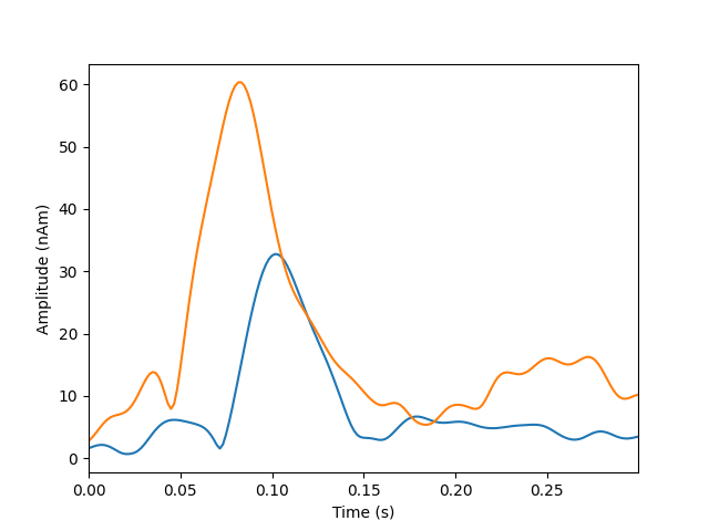
Plot dipole activations
plot_dipole_amplitudes(dipoles)
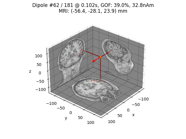
# Plot dipole location of the strongest dipole with MRI slices
idx = np.argmax([np.max(np.abs(dip.amplitude)) for dip in dipoles])
plot_dipole_locations(dipoles[idx], forward['mri_head_t'], 'sample',
subjects_dir=subjects_dir, mode='orthoview',
idx='amplitude')
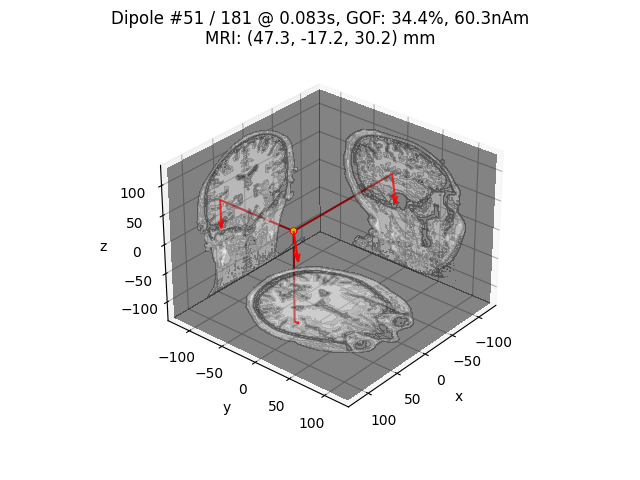
# Plot dipole locations of all dipoles with MRI slices
for dip in dipoles:
plot_dipole_locations(dip, forward['mri_head_t'], 'sample',
subjects_dir=subjects_dir, mode='orthoview',
idx='amplitude')

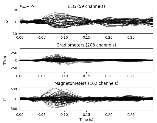
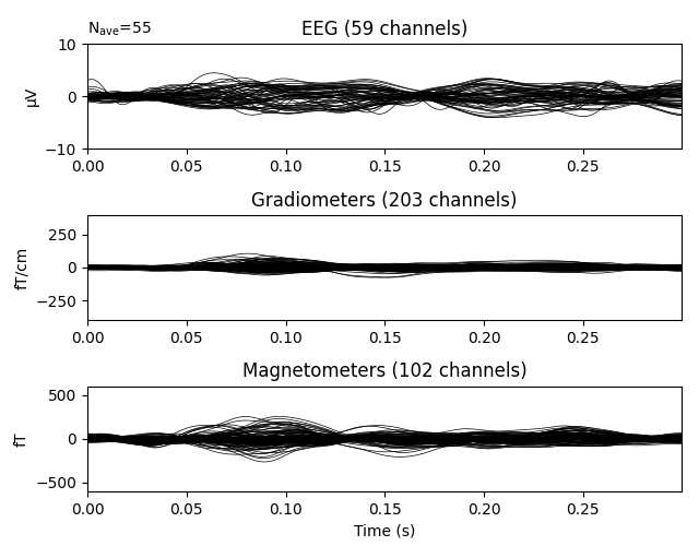
Plot residual
ylim = dict(eeg=[-10, 10], grad=[-400, 400], mag=[-600, 600])
evoked.pick_types(meg=True, eeg=True, exclude='bads')
evoked.plot(ylim=ylim, proj=True, time_unit='s')
residual.pick_types(meg=True, eeg=True, exclude='bads')
residual.plot(ylim=ylim, proj=True, time_unit='s')
Generate stc from dipoles
stc = make_stc_from_dipoles(dipoles, forward['src'])
Out:
Converting dipoles into a SourceEstimate.
[done]
View in 2D and 3D (“glass” brain like 3D plot)
solver = "MxNE" if n_mxne_iter == 1 else "irMxNE"
plot_sparse_source_estimates(forward['src'], stc, bgcolor=(1, 1, 1),
                             fig_name="%s (cond %s)" % (solver, condition),
                             opacity=0.1)
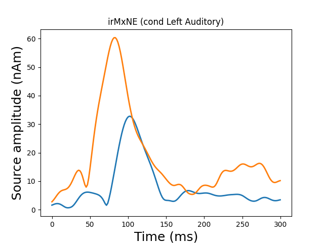
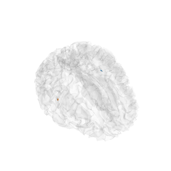
Out:
Total number of active sources: 2
Morph onto fsaverage brain and view
morph = mne.compute_source_morph(stc, subject_from='sample',
                                 subject_to='fsaverage', spacing=None,
                                 sparse=True, subjects_dir=subjects_dir)
stc_fsaverage = morph.apply(stc)
src_fsaverage_fname = subjects_dir + '/fsaverage/bem/fsaverage-ico-5-src.fif'
src_fsaverage = mne.read_source_spaces(src_fsaverage_fname)

plot_sparse_source_estimates(src_fsaverage, stc_fsaverage, bgcolor=(1, 1, 1),
                             fig_name="Morphed %s (cond %s)" % (solver,
                             condition), opacity=0.1)
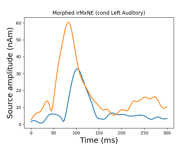
Out:
    Reading a source space...
    [done]
    Reading a source space...
    [done]
    2 source spaces read
Total number of active sources: 2
References
- 1
Alexandre Gramfort, Matthieu Kowalski, and Matti S. Hämäläinen. Mixed-norm estimates for the M/EEG inverse problem using accelerated gradient methods. Physics in Medicine and Biology, 57(7):1937–1961, 2012. doi:10.1088/0031-9155/57/7/1937.
- 2
Daniel Strohmeier, Jens Haueisen, and Alexandre Gramfort. Improved MEG/EEG source localization with reweighted mixed-norms. In Proceedings of PRNI-2014, 1–4. Tübingen, 2014. IEEE. doi:10.1109/PRNI.2014.6858545.
Total running time of the script: ( 0 minutes 21.701 seconds)
Estimated memory usage: 349 MB