Note
Click here to download the full example code
Compute iterative reweighted TF-MxNE with multiscale time-frequency dictionary
The iterative reweighted TF-MxNE solver is a distributed inverse method based on the TF-MxNE solver, which promotes focal (sparse) sources 1. The benefit of this approach is that:
it is spatio-temporal without assuming stationarity (sources properties can vary over time),
activations are localized in space, time and frequency in one step,
the solver uses non-convex penalties in the TF domain, which results in a solution less biased towards zero than when simple TF-MxNE is used,
using a multiscale dictionary allows to capture short transient activations along with slower brain waves 2.
# Author: Mathurin Massias <mathurin.massias@gmail.com>
#         Yousra Bekhti <yousra.bekhti@gmail.com>
#         Daniel Strohmeier <daniel.strohmeier@tu-ilmenau.de>
#         Alexandre Gramfort <alexandre.gramfort@inria.fr>
#
# License: BSD (3-clause)

import os.path as op

import mne
from mne.datasets import somato
from mne.inverse_sparse import tf_mixed_norm, make_stc_from_dipoles
from mne.viz import plot_sparse_source_estimates

print(__doc__)
Load somatosensory MEG data
data_path = somato.data_path()
subject = '01'
task = 'somato'
raw_fname = op.join(data_path, 'sub-{}'.format(subject), 'meg',
                    'sub-{}_task-{}_meg.fif'.format(subject, task))
fwd_fname = op.join(data_path, 'derivatives', 'sub-{}'.format(subject),
                    'sub-{}_task-{}-fwd.fif'.format(subject, task))

condition = 'Unknown'

# Read evoked
raw = mne.io.read_raw_fif(raw_fname)
events = mne.find_events(raw, stim_channel='STI 014')
reject = dict(grad=4000e-13, eog=350e-6)
picks = mne.pick_types(raw.info, meg=True, eog=True)

event_id, tmin, tmax = 1, -1., 3.
epochs = mne.Epochs(raw, events, event_id, tmin, tmax, picks=picks,
                    reject=reject, preload=True)
evoked = epochs.filter(1, None).average()
evoked = evoked.pick_types(meg=True)
evoked.crop(tmin=0.008, tmax=0.2)

# Compute noise covariance matrix
cov = mne.compute_covariance(epochs, rank='info', tmax=0.)

# Handling forward solution
forward = mne.read_forward_solution(fwd_fname)
Out:
Opening raw data file /home/circleci/mne_data/MNE-somato-data/sub-01/meg/sub-01_task-somato_meg.fif...
    Range : 237600 ... 506999 =    791.189 ...  1688.266 secs
Ready.
111 events found
Event IDs: [1]
Not setting metadata
Not setting metadata
111 matching events found
Setting baseline interval to [-0.9989760657919393, 0.0] sec
Applying baseline correction (mode: mean)
0 projection items activated
Loading data for 111 events and 1202 original time points ...
    Rejecting  epoch based on EOG : ['EOG 061']
    Rejecting  epoch based on EOG : ['EOG 061']
    Rejecting  epoch based on EOG : ['EOG 061']
3 bad epochs dropped
Setting up high-pass filter at 1 Hz

FIR filter parameters
---------------------
Designing a one-pass, zero-phase, non-causal highpass filter:
- Windowed time-domain design (firwin) method
- Hamming window with 0.0194 passband ripple and 53 dB stopband attenuation
- Lower passband edge: 1.00
- Lower transition bandwidth: 1.00 Hz (-6 dB cutoff frequency: 0.50 Hz)
- Filter length: 993 samples (3.307 sec)

Computing rank from data with rank='info'
    MEG: rank 64 after 0 projectors applied to 306 channels
    Setting small MEG eigenvalues to zero (without PCA)
Reducing data rank from 306 -> 64
Estimating covariance using EMPIRICAL
Done.
Number of samples used : 32508
[done]
Reading forward solution from /home/circleci/mne_data/MNE-somato-data/derivatives/sub-01/sub-01_task-somato-fwd.fif...
    Reading a source space...
    [done]
    Reading a source space...
    [done]
    2 source spaces read
    Desired named matrix (kind = 3523) not available
    Read MEG forward solution (8155 sources, 306 channels, free orientations)
    Source spaces transformed to the forward solution coordinate frame
Run iterative reweighted multidict TF-MxNE solver
alpha, l1_ratio = 20, 0.05
loose, depth = 1, 0.95
# Use a multiscale time-frequency dictionary
wsize, tstep = [4, 16], [2, 4]


n_tfmxne_iter = 10
# Compute TF-MxNE inverse solution with dipole output
dipoles, residual = tf_mixed_norm(
    evoked, forward, cov, alpha=alpha, l1_ratio=l1_ratio,
    n_tfmxne_iter=n_tfmxne_iter, loose=loose,
    depth=depth, tol=1e-3,
    wsize=wsize, tstep=tstep, return_as_dipoles=True,
    return_residual=True)

# Crop to remove edges
for dip in dipoles:
    dip.crop(tmin=-0.05, tmax=0.3)
evoked.crop(tmin=-0.05, tmax=0.3)
residual.crop(tmin=-0.05, tmax=0.3)
Out:
Computing inverse operator with 306 channels.
    306 out of 306 channels remain after picking
Selected 306 channels
Creating the depth weighting matrix...
Whitening the forward solution.
Computing rank from covariance with rank=None
    Using tolerance 3.8e-12 (2.2e-16 eps * 306 dim * 55  max singular value)
    Estimated rank (mag + grad): 64
    MEG: rank 64 computed from 306 data channels with 0 projectors
    Setting small MEG eigenvalues to zero (without PCA)
Creating the source covariance matrix
Adjusting source covariance matrix.
Whitening data matrix.

dgap 5.30e+01 :: p_obj 219.111438 :: d_obj 166.093924 :: n_active 187

dgap 1.26e+01 :: p_obj 207.829965 :: d_obj 195.192651 :: n_active 146

    Iteration 10 :: n_active 109
    dgap 1.96e+00 :: p_obj 206.332222 :: d_obj 204.372084

dgap 2.00e+00 :: p_obj 206.173555 :: d_obj 204.174517 :: n_active 91

    Iteration 10 :: n_active 79
    dgap 1.19e+00 :: p_obj 206.053443 :: d_obj 204.866068

    Iteration 20 :: n_active 68
    dgap 8.96e-01 :: p_obj 205.998619 :: d_obj 205.102729

    Iteration 30 :: n_active 63
    dgap 6.79e-01 :: p_obj 205.958722 :: d_obj 205.279576

dgap 6.79e-01 :: p_obj 205.958722 :: d_obj 205.279576 :: n_active 63

Convergence reached!

Iteration 1: active set size=63, E=716.228469

    Iteration 10 :: n_active 12
    dgap 3.63e+00 :: p_obj 259.829107 :: d_obj 256.199601

    Iteration 20 :: n_active 12
    dgap 2.45e+00 :: p_obj 259.550599 :: d_obj 257.102324

    Iteration 30 :: n_active 11
    dgap 8.95e-01 :: p_obj 259.447620 :: d_obj 258.552132

    Iteration 40 :: n_active 11
    dgap 5.70e-01 :: p_obj 259.401046 :: d_obj 258.831477

dgap 5.70e-01 :: p_obj 259.401046 :: d_obj 258.831477 :: n_active 11

Convergence reached!

Iteration 2: active set size=11, E=322.858183

    Iteration 10 :: n_active 6
    dgap 2.37e+00 :: p_obj 221.951597 :: d_obj 219.582361

    Iteration 20 :: n_active 5
    dgap 3.74e-01 :: p_obj 221.820898 :: d_obj 221.447360

dgap 3.74e-01 :: p_obj 221.820898 :: d_obj 221.447360 :: n_active 5

Convergence reached!

Iteration 3: active set size=5, E=263.705321

    Iteration 10 :: n_active 4
    dgap 5.41e-01 :: p_obj 202.744185 :: d_obj 202.203575

dgap 5.41e-01 :: p_obj 202.744185 :: d_obj 202.203575 :: n_active 4

Convergence reached!

Iteration 4: active set size=4, E=257.598857

    Iteration 10 :: n_active 4
    dgap 4.13e-01 :: p_obj 199.013542 :: d_obj 198.600553

dgap 4.13e-01 :: p_obj 199.013542 :: d_obj 198.600553 :: n_active 4

Convergence reached!

Iteration 5: active set size=4, E=256.932103
Convergence reached after 4 reweightings!
Debiasing converged after 276 iterations max(|D - D0| = 7.775514e-07 < 1.000000e-06)
[done]
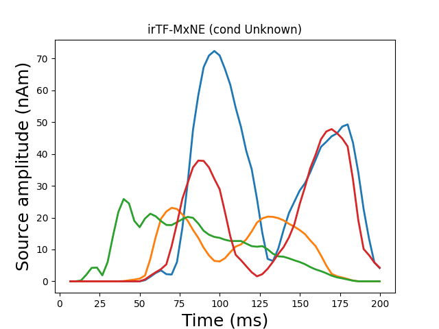
Generate stc from dipoles
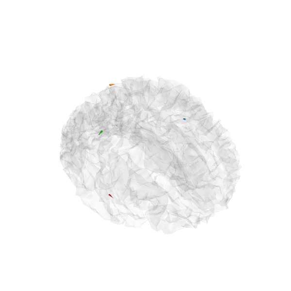
stc = make_stc_from_dipoles(dipoles, forward['src'])

plot_sparse_source_estimates(forward['src'], stc, bgcolor=(1, 1, 1),
                             opacity=0.1, fig_name="irTF-MxNE (cond %s)"
                             % condition)


Out:
Converting dipoles into a SourceEstimate.
[done]
Total number of active sources: 4
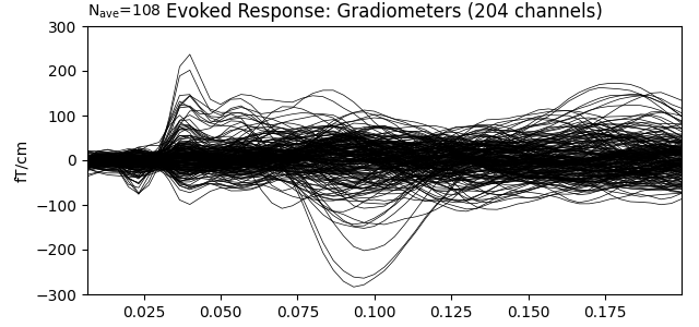
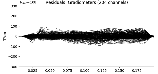
Show the evoked response and the residual for gradiometers
ylim = dict(grad=[-300, 300])
evoked.pick_types(meg='grad')
evoked.plot(titles=dict(grad='Evoked Response: Gradiometers'), ylim=ylim,
            proj=True)

residual.pick_types(meg='grad')
residual.plot(titles=dict(grad='Residuals: Gradiometers'), ylim=ylim,
              proj=True)
References
- 1
Daniel Strohmeier, Alexandre Gramfort, and Jens Haueisen. MEG/EEG Source Imaging with a Non-Convex Penalty in the Time-Frequency Domain. In 2015 International Workshop on Pattern Recognition in NeuroImaging, 21–24. June 2015. doi:10.1109/PRNI.2015.14.
- 2
Yousra Bekhti, Daniel Strohmeiery, Mainak Jas, Roland Badeau, and Alexandre Gramfort. M/EEG source localization with multi-scale time-frequency dictionaries. In Proceedings of PRNI-2016, 1–4. Trento, 2016. IEEE. doi:10.1109/PRNI.2016.7552337.
Total running time of the script: ( 1 minutes 25.927 seconds)
Estimated memory usage: 667 MB

