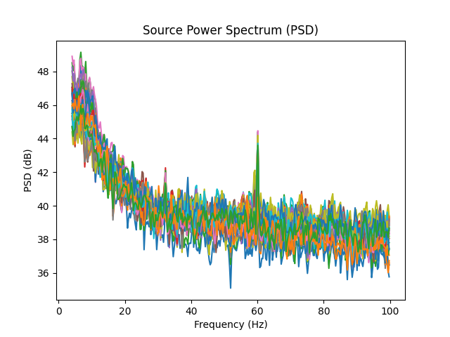
Compute source power spectral density (PSD) in a label¶

Returns an STC file containing the PSD (in dB) of each of the sources within a label.

# Authors: Alexandre Gramfort <alexandre.gramfort@inria.fr>
#
# License: BSD (3-clause)

import matplotlib.pyplot as plt

import mne
from mne import io
from mne.datasets import sample
from mne.minimum_norm import read_inverse_operator, compute_source_psd

print(__doc__)

Set parameters

data_path = sample.data_path()
raw_fname = data_path + '/MEG/sample/sample_audvis_raw.fif'
fname_inv = data_path + '/MEG/sample/sample_audvis-meg-oct-6-meg-inv.fif'
fname_label = data_path + '/MEG/sample/labels/Aud-lh.label'

# Setup for reading the raw data
raw = io.read_raw_fif(raw_fname, verbose=False)
events = mne.find_events(raw, stim_channel='STI 014')
inverse_operator = read_inverse_operator(fname_inv)
raw.info['bads'] = ['MEG 2443', 'EEG 053']

# picks MEG gradiometers
picks = mne.pick_types(raw.info, meg=True, eeg=False, eog=True,
                       stim=False, exclude='bads')

tmin, tmax = 0, 120  # use the first 120s of data
fmin, fmax = 4, 100  # look at frequencies between 4 and 100Hz
n_fft = 2048  # the FFT size (n_fft). Ideally a power of 2
label = mne.read_label(fname_label)

stc = compute_source_psd(raw, inverse_operator, lambda2=1. / 9., method="dSPM",
                         tmin=tmin, tmax=tmax, fmin=fmin, fmax=fmax,
                         pick_ori="normal", n_fft=n_fft, label=label,
                         dB=True)

stc.save('psd_dSPM')

Out:

320 events found
Event IDs: [ 1  2  3  4  5 32]
Reading inverse operator decomposition from /home/circleci/mne_data/MNE-sample-data/MEG/sample/sample_audvis-meg-oct-6-meg-inv.fif...
    Reading inverse operator info...
    [done]
    Reading inverse operator decomposition...
    [done]
    305 x 305 full covariance (kind = 1) found.
    Read a total of 4 projection items:
        PCA-v1 (1 x 102) active
        PCA-v2 (1 x 102) active
        PCA-v3 (1 x 102) active
        Average EEG reference (1 x 60) active
    Noise covariance matrix read.
    22494 x 22494 diagonal covariance (kind = 2) found.
    Source covariance matrix read.
    22494 x 22494 diagonal covariance (kind = 6) found.
    Orientation priors read.
    22494 x 22494 diagonal covariance (kind = 5) found.
    Depth priors read.
    Did not find the desired covariance matrix (kind = 3)
    Reading a source space...
    Computing patch statistics...
    Patch information added...
    Distance information added...
    [done]
    Reading a source space...
    Computing patch statistics...
    Patch information added...
    Distance information added...
    [done]
    2 source spaces read
    Read a total of 4 projection items:
        PCA-v1 (1 x 102) active
        PCA-v2 (1 x 102) active
        PCA-v3 (1 x 102) active
        Average EEG reference (1 x 60) active
    Source spaces transformed to the inverse solution coordinate frame
Not setting metadata
Not setting metadata
70 matching events found
No baseline correction applied
Created an SSP operator (subspace dimension = 3)
3 projection items activated
Considering frequencies 4 ... 100 Hz
Preparing the inverse operator for use...
    Scaled noise and source covariance from nave = 1 to nave = 1
    Created the regularized inverter
    Created an SSP operator (subspace dimension = 3)
    Created the whitener using a noise covariance matrix with rank 302 (3 small eigenvalues omitted)
    Computing noise-normalization factors (dSPM)...
[done]
Picked 305 channels from the data
Computing inverse...
    Eigenleads need to be weighted ...
Reducing data rank 33 -> 33
Using hann windowing on at most 70 epochs

  0%|          |  : 0/70 [00:00<?,       ?it/s]
  1%|1         |  : 1/70 [00:00<00:07,    9.60it/s]
  3%|2         |  : 2/70 [00:00<00:06,   10.32it/s]
  4%|4         |  : 3/70 [00:00<00:04,   14.18it/s]
  6%|5         |  : 4/70 [00:00<00:04,   13.88it/s]
  7%|7         |  : 5/70 [00:00<00:03,   16.30it/s]
  9%|8         |  : 6/70 [00:00<00:04,   15.37it/s]
 10%|#         |  : 7/70 [00:00<00:03,   17.30it/s]
 11%|#1        |  : 8/70 [00:00<00:03,   16.53it/s]
 13%|#2        |  : 9/70 [00:00<00:03,   18.06it/s]
 14%|#4        |  : 10/70 [00:00<00:03,   17.23it/s]
 16%|#5        |  : 11/70 [00:00<00:03,   18.59it/s]
 17%|#7        |  : 12/70 [00:00<00:03,   17.63it/s]
 19%|#8        |  : 13/70 [00:00<00:03,   18.81it/s]
 20%|##        |  : 14/70 [00:00<00:03,   18.04it/s]
 21%|##1       |  : 15/70 [00:00<00:02,   19.13it/s]
 23%|##2       |  : 16/70 [00:00<00:02,   18.36it/s]
 24%|##4       |  : 17/70 [00:00<00:02,   19.33it/s]
 26%|##5       |  : 18/70 [00:00<00:02,   18.61it/s]
 27%|##7       |  : 19/70 [00:01<00:02,   19.49it/s]
 29%|##8       |  : 20/70 [00:01<00:02,   18.77it/s]
 30%|###       |  : 21/70 [00:01<00:02,   19.63it/s]
 31%|###1      |  : 22/70 [00:01<00:02,   18.83it/s]
 33%|###2      |  : 23/70 [00:01<00:02,   19.67it/s]
 34%|###4      |  : 24/70 [00:01<00:02,   18.88it/s]
 36%|###5      |  : 25/70 [00:01<00:02,   19.69it/s]
 37%|###7      |  : 26/70 [00:01<00:02,   18.92it/s]
 39%|###8      |  : 27/70 [00:01<00:02,   19.70it/s]
 40%|####      |  : 28/70 [00:01<00:02,   18.96it/s]
 41%|####1     |  : 29/70 [00:01<00:02,   18.42it/s]
 43%|####2     |  : 30/70 [00:01<00:02,   19.04it/s]
 44%|####4     |  : 31/70 [00:01<00:02,   18.57it/s]
 46%|####5     |  : 32/70 [00:01<00:01,   19.18it/s]
 47%|####7     |  : 33/70 [00:01<00:01,   18.71it/s]
 49%|####8     |  : 34/70 [00:01<00:01,   19.30it/s]
 50%|#####     |  : 35/70 [00:01<00:01,   18.83it/s]
 51%|#####1    |  : 36/70 [00:01<00:01,   19.39it/s]
 53%|#####2    |  : 37/70 [00:01<00:01,   18.85it/s]
 54%|#####4    |  : 38/70 [00:02<00:01,   19.44it/s]
 56%|#####5    |  : 39/70 [00:02<00:01,   18.87it/s]
 57%|#####7    |  : 40/70 [00:02<00:01,   19.49it/s]
 59%|#####8    |  : 41/70 [00:02<00:01,   18.92it/s]
 60%|######    |  : 42/70 [00:02<00:01,   19.55it/s]
 61%|######1   |  : 43/70 [00:02<00:01,   18.94it/s]
 63%|######2   |  : 44/70 [00:02<00:01,   19.55it/s]
 64%|######4   |  : 45/70 [00:02<00:01,   18.93it/s]
 66%|######5   |  : 46/70 [00:02<00:01,   19.56it/s]
 67%|######7   |  : 47/70 [00:02<00:01,   19.04it/s]
 69%|######8   |  : 48/70 [00:02<00:01,   19.66it/s]
 70%|#######   |  : 49/70 [00:02<00:01,   19.12it/s]
 71%|#######1  |  : 50/70 [00:02<00:01,   19.71it/s]
 73%|#######2  |  : 51/70 [00:02<00:00,   19.19it/s]
 74%|#######4  |  : 52/70 [00:02<00:00,   19.81it/s]
 76%|#######5  |  : 53/70 [00:02<00:00,   19.19it/s]
 77%|#######7  |  : 54/70 [00:02<00:00,   19.81it/s]
 79%|#######8  |  : 55/70 [00:02<00:00,   19.29it/s]
 80%|########  |  : 56/70 [00:02<00:00,   19.91it/s]
 81%|########1 |  : 57/70 [00:02<00:00,   19.28it/s]
 83%|########2 |  : 58/70 [00:03<00:00,   19.89it/s]
 84%|########4 |  : 59/70 [00:03<00:00,   19.35it/s]
 86%|########5 |  : 60/70 [00:03<00:00,   19.96it/s]
 87%|########7 |  : 61/70 [00:03<00:00,   19.30it/s]
 89%|########8 |  : 62/70 [00:03<00:00,   19.91it/s]
 90%|######### |  : 63/70 [00:03<00:00,   19.36it/s]
 91%|#########1|  : 64/70 [00:03<00:00,   19.94it/s]
 93%|#########2|  : 65/70 [00:03<00:00,   19.38it/s]
 94%|#########4|  : 66/70 [00:03<00:00,   19.98it/s]
 96%|#########5|  : 67/70 [00:03<00:00,   19.43it/s]
 97%|#########7|  : 68/70 [00:03<00:00,   20.03it/s]
 99%|#########8|  : 69/70 [00:03<00:00,   19.41it/s]
100%|##########|  : 70/70 [00:03<00:00,   18.92it/s]
100%|##########|  : 70/70 [00:03<00:00,   19.03it/s]
Writing STC to disk...
[done]

View PSD of sources in label

plt.plot(stc.times, stc.data.T)
plt.xlabel('Frequency (Hz)')
plt.ylabel('PSD (dB)')
plt.title('Source Power Spectrum (PSD)')
plt.show()

Total running time of the script: ( 0 minutes 8.994 seconds)

Estimated memory usage: 8 MB

Gallery generated by Sphinx-Gallery