Temporal whitening with AR model¶

Here we fit an AR model to the data and use it to temporally whiten the signals.

# Authors: Alexandre Gramfort <alexandre.gramfort@inria.fr>
#
# License: BSD (3-clause)

import numpy as np
from scipy import signal
import matplotlib.pyplot as plt

import mne
from mne.time_frequency import fit_iir_model_raw
from mne.datasets import sample

print(__doc__)

data_path = sample.data_path()

raw_fname = data_path + '/MEG/sample/sample_audvis_raw.fif'
proj_fname = data_path + '/MEG/sample/sample_audvis_ecg-proj.fif'

raw = mne.io.read_raw_fif(raw_fname)
proj = mne.read_proj(proj_fname)
raw.info['projs'] += proj
raw.info['bads'] = ['MEG 2443', 'EEG 053']  # mark bad channels

# Set up pick list: Gradiometers - bad channels
picks = mne.pick_types(raw.info, meg='grad', exclude='bads')

order = 5  # define model order
picks = picks[:1]

# Estimate AR models on raw data
b, a = fit_iir_model_raw(raw, order=order, picks=picks, tmin=60, tmax=180)
d, times = raw[0, 10000:20000]  # look at one channel from now on
d = d.ravel()  # make flat vector
innovation = signal.convolve(d, a, 'valid')
d_ = signal.lfilter(b, a, innovation)  # regenerate the signal
d_ = np.r_[d_[0] * np.ones(order), d_]  # dummy samples to keep signal length

Out:

Opening raw data file /home/circleci/mne_data/MNE-sample-data/MEG/sample/sample_audvis_raw.fif...
    Read a total of 3 projection items:
        PCA-v1 (1 x 102)  idle
        PCA-v2 (1 x 102)  idle
        PCA-v3 (1 x 102)  idle
    Range : 25800 ... 192599 =     42.956 ...   320.670 secs
Ready.
    Read a total of 6 projection items:
        ECG-planar-999--0.200-0.400-PCA-01 (1 x 203)  idle
        ECG-planar-999--0.200-0.400-PCA-02 (1 x 203)  idle
        ECG-axial-999--0.200-0.400-PCA-01 (1 x 102)  idle
        ECG-axial-999--0.200-0.400-PCA-02 (1 x 102)  idle
        ECG-eeg-999--0.200-0.400-PCA-01 (1 x 59)  idle
        ECG-eeg-999--0.200-0.400-PCA-02 (1 x 59)  idle

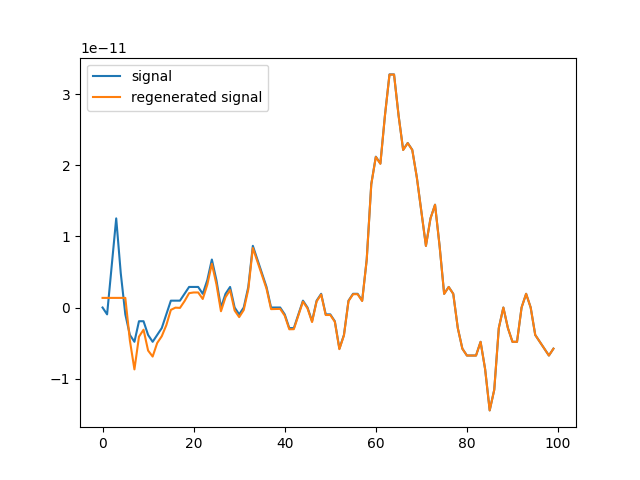
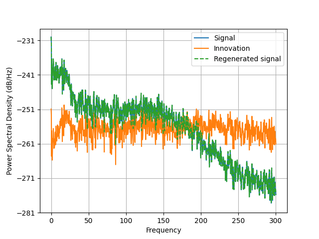
Plot the different time series and PSDs

plt.close('all')
plt.figure()
plt.plot(d[:100], label='signal')
plt.plot(d_[:100], label='regenerated signal')
plt.legend()

plt.figure()
plt.psd(d, Fs=raw.info['sfreq'], NFFT=2048)
plt.psd(innovation, Fs=raw.info['sfreq'], NFFT=2048)
plt.psd(d_, Fs=raw.info['sfreq'], NFFT=2048, linestyle='--')
plt.legend(('Signal', 'Innovation', 'Regenerated signal'))
plt.show()