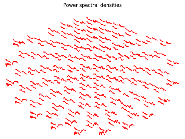
Plot custom topographies for MEG sensors¶

This example exposes the iter_topography() function that makes it very easy to generate custom sensor topography plots. Here we will plot the power spectrum of each channel on a topographic layout.

Out:

Opening raw data file /home/circleci/mne_data/MNE-sample-data/MEG/sample/sample_audvis_filt-0-40_raw.fif...
    Read a total of 4 projection items:
        PCA-v1 (1 x 102)  idle
        PCA-v2 (1 x 102)  idle
        PCA-v3 (1 x 102)  idle
        Average EEG reference (1 x 60)  idle
    Range : 6450 ... 48149 =     42.956 ...   320.665 secs
Ready.
Reading 0 ... 41699  =      0.000 ...   277.709 secs...
Filtering raw data in 1 contiguous segment
Setting up band-pass filter from 1 - 20 Hz

FIR filter parameters
---------------------
Designing a one-pass, zero-phase, non-causal bandpass filter:
- Windowed time-domain design (firwin) method
- Hamming window with 0.0194 passband ripple and 53 dB stopband attenuation
- Lower passband edge: 1.00
- Lower transition bandwidth: 1.00 Hz (-6 dB cutoff frequency: 0.50 Hz)
- Upper passband edge: 20.00 Hz
- Upper transition bandwidth: 5.00 Hz (-6 dB cutoff frequency: 22.50 Hz)
- Filter length: 497 samples (3.310 sec)

Effective window size : 1.705 (s)

# Author: Denis A. Engemann <denis.engemann@gmail.com>
#
# License: BSD (3-clause)


import numpy as np
import matplotlib.pyplot as plt

import mne
from mne.viz import iter_topography
from mne import io
from mne.time_frequency import psd_welch
from mne.datasets import sample

print(__doc__)

data_path = sample.data_path()
raw_fname = data_path + '/MEG/sample/sample_audvis_filt-0-40_raw.fif'

raw = io.read_raw_fif(raw_fname, preload=True)
raw.filter(1, 20, fir_design='firwin')

picks = mne.pick_types(raw.info, meg=True, exclude=[])
tmin, tmax = 0, 120  # use the first 120s of data
fmin, fmax = 2, 20  # look at frequencies between 2 and 20Hz
n_fft = 2048  # the FFT size (n_fft). Ideally a power of 2
psds, freqs = psd_welch(raw, picks=picks, tmin=tmin, tmax=tmax,
                        fmin=fmin, fmax=fmax)
psds = 20 * np.log10(psds)  # scale to dB


def my_callback(ax, ch_idx):
    """
    This block of code is executed once you click on one of the channel axes
    in the plot. To work with the viz internals, this function should only take
    two parameters, the axis and the channel or data index.
    """
    ax.plot(freqs, psds[ch_idx], color='red')
    ax.set_xlabel('Frequency (Hz)')
    ax.set_ylabel('Power (dB)')


for ax, idx in iter_topography(raw.info,
                               fig_facecolor='white',
                               axis_facecolor='white',
                               axis_spinecolor='white',
                               on_pick=my_callback):
    ax.plot(psds[idx], color='red')

plt.gcf().suptitle('Power spectral densities')
plt.show()