Note
Click here to download the full example code
Working with ECoG data
MNE supports working with more than just MEG and EEG data. Here we show some of the functions that can be used to facilitate working with electrocorticography (ECoG) data.
This example shows how to use:
ECoG data
channel locations in subject’s MRI space
projection onto a surface
For an example that involves sEEG data, channel locations in MNI space, or projection into a volume, see Working with sEEG data.
# Authors: Eric Larson <larson.eric.d@gmail.com>
# Chris Holdgraf <choldgraf@gmail.com>
# Adam Li <adam2392@gmail.com>
#
# License: BSD (3-clause)
import pandas as pd
import numpy as np
import matplotlib.pyplot as plt
import matplotlib.animation as animation
import mne
from mne.viz import plot_alignment, snapshot_brain_montage
print(__doc__)
# paths to mne datasets - sample ECoG and FreeSurfer subject
misc_path = mne.datasets.misc.data_path()
sample_path = mne.datasets.sample.data_path()
subject = 'sample'
subjects_dir = sample_path + '/subjects'
Let’s load some ECoG electrode locations and names, and turn them into
a mne.channels.DigMontage class. First, use pandas to read in the
.tsv file.
# In this tutorial, the electrode coordinates are assumed to be in meters
elec_df = pd.read_csv(misc_path + '/ecog/sample_ecog_electrodes.tsv',
sep='\t', header=0, index_col=None)
ch_names = elec_df['name'].tolist()
ch_coords = elec_df[['x', 'y', 'z']].to_numpy(dtype=float)
ch_pos = dict(zip(ch_names, ch_coords))
# Ideally the nasion/LPA/RPA will also be present from the digitization, here
# we use fiducials estimated from the subject's FreeSurfer MNI transformation:
lpa, nasion, rpa = mne.coreg.get_mni_fiducials(
subject, subjects_dir=subjects_dir)
lpa, nasion, rpa = lpa['r'], nasion['r'], rpa['r']
Now we make a mne.channels.DigMontage stating that the ECoG
contacts are in the FreeSurfer surface RAS (i.e., MRI) coordinate system.
Out:
Created 64 channel positions
Now we get the trans that transforms from our MRI coordinate system
to the head coordinate frame. This transform will be applied to the
data when applying the montage so that standard plotting functions like
mne.viz.plot_evoked_topomap() will be aligned properly.
trans = mne.channels.compute_native_head_t(montage)
print(trans)
Out:
<Transform | MRI (surface RAS)->head>
[[ 0.99771797 -0.05883969 -0.03311713 0.00461628]
[ 0.0673865 0.89849754 0.43377555 0.00599143]
[ 0.00423244 -0.4350173 0.90041215 0.0066259 ]
[ 0. 0. 0. 1. ]]
Now that we have our montage, we can load in our corresponding time-series data and set the montage to the raw data.
# first we'll load in the sample dataset
raw = mne.io.read_raw_edf(misc_path + '/ecog/sample_ecog.edf')
# drop bad channels
raw.info['bads'].extend([ch for ch in raw.ch_names if ch not in ch_names])
raw.load_data()
raw.drop_channels(raw.info['bads'])
raw.crop(0, 2) # just process 2 sec of data for speed
# attach montage
raw.set_montage(montage)
# set channel types to ECoG (instead of EEG)
raw.set_channel_types({ch_name: 'ecog' for ch_name in raw.ch_names})
Out:
Extracting EDF parameters from /home/circleci/mne_data/MNE-misc-data/ecog/sample_ecog.edf...
EDF file detected
Setting channel info structure...
Creating raw.info structure...
Reading 0 ... 21657 = 0.000 ... 21.670 secs...
We can then plot the locations of our electrodes on our subject’s brain.
We’ll use snapshot_brain_montage() to save the plot as image
data (along with xy positions of each electrode in the image), so that later
we can plot frequency band power on top of it.
Note
These are not real electrodes for this subject, so they do not align to the cortical surface perfectly.
fig = plot_alignment(raw.info, subject=subject, subjects_dir=subjects_dir,
surfaces=['pial'], trans=trans, coord_frame='mri')
mne.viz.set_3d_view(fig, 200, 70, focalpoint=[0, -0.005, 0.03])
xy, im = snapshot_brain_montage(fig, montage)
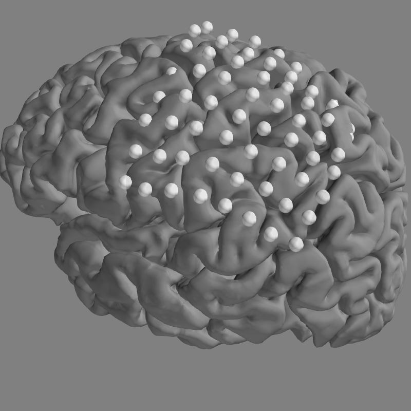
Out:
Plotting 64 ECoG locations
Next, we’ll compute the signal power in the gamma (30-90 Hz) and alpha (8-12 Hz) bands.
gamma_power_t = raw.copy().filter(30, 90).apply_hilbert(
envelope=True).get_data()
alpha_power_t = raw.copy().filter(8, 12).apply_hilbert(
envelope=True).get_data()
gamma_power = gamma_power_t.mean(axis=-1)
alpha_power = alpha_power_t.mean(axis=-1)
Out:
Filtering raw data in 1 contiguous segment
Setting up band-pass filter from 30 - 90 Hz
FIR filter parameters
---------------------
Designing a one-pass, zero-phase, non-causal bandpass filter:
- Windowed time-domain design (firwin) method
- Hamming window with 0.0194 passband ripple and 53 dB stopband attenuation
- Lower passband edge: 30.00
- Lower transition bandwidth: 7.50 Hz (-6 dB cutoff frequency: 26.25 Hz)
- Upper passband edge: 90.00 Hz
- Upper transition bandwidth: 22.50 Hz (-6 dB cutoff frequency: 101.25 Hz)
- Filter length: 441 samples (0.441 sec)
Filtering raw data in 1 contiguous segment
Setting up band-pass filter from 8 - 12 Hz
FIR filter parameters
---------------------
Designing a one-pass, zero-phase, non-causal bandpass filter:
- Windowed time-domain design (firwin) method
- Hamming window with 0.0194 passband ripple and 53 dB stopband attenuation
- Lower passband edge: 8.00
- Lower transition bandwidth: 2.00 Hz (-6 dB cutoff frequency: 7.00 Hz)
- Upper passband edge: 12.00 Hz
- Upper transition bandwidth: 3.00 Hz (-6 dB cutoff frequency: 13.50 Hz)
- Filter length: 1651 samples (1.652 sec)
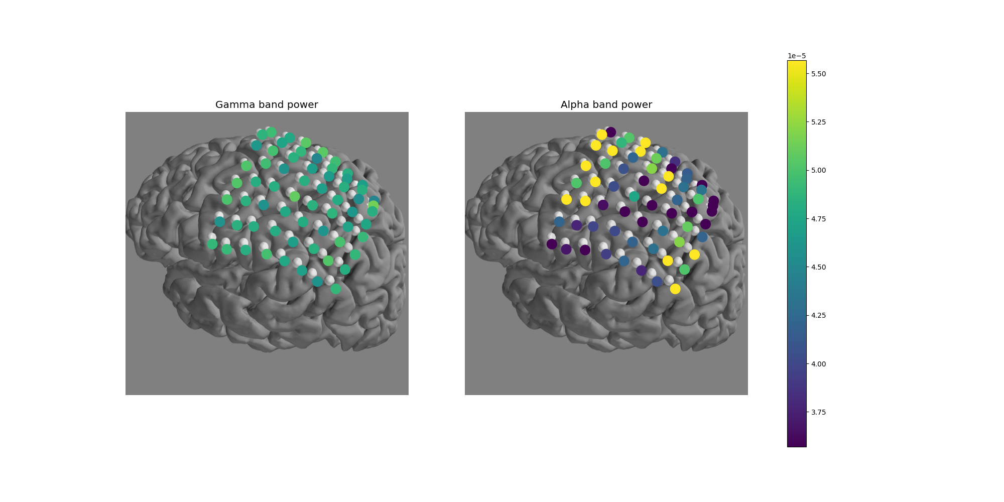
Now let’s use matplotlib to overplot frequency band power onto the electrodes
which can be plotted on top of the brain from
snapshot_brain_montage().
# Convert from a dictionary to array to plot
xy_pts = np.vstack([xy[ch] for ch in raw.info['ch_names']])
# colormap to view spectral power
cmap = 'viridis'
# Create a 1x2 figure showing the average power in gamma and alpha bands.
fig, axs = plt.subplots(1, 2, figsize=(20, 10))
# choose a colormap range wide enough for both frequency bands
_gamma_alpha_power = np.concatenate((gamma_power, alpha_power)).flatten()
vmin, vmax = np.percentile(_gamma_alpha_power, [10, 90])
for ax, band_power, band in zip(axs,
[gamma_power, alpha_power],
['Gamma', 'Alpha']):
ax.imshow(im)
ax.set_axis_off()
sc = ax.scatter(*xy_pts.T, c=band_power, s=200,
cmap=cmap, vmin=vmin, vmax=vmax)
ax.set_title(f'{band} band power', size='x-large')
fig.colorbar(sc, ax=axs)
Say we want to visualize the evolution of the power in the gamma band,
instead of just plotting the average. We can use
matplotlib.animation.FuncAnimation to create an animation and apply this
to the brain figure.
# create an initialization and animation function
# to pass to FuncAnimation
def init():
"""Create an empty frame."""
return paths,
def animate(i, activity):
"""Animate the plot."""
paths.set_array(activity[:, i])
return paths,
# create the figure and apply the animation of the
# gamma frequency band activity
fig, ax = plt.subplots(figsize=(5, 5))
ax.imshow(im)
ax.set_axis_off()
paths = ax.scatter(*xy_pts.T, c=np.zeros(len(xy_pts)), s=200,
cmap=cmap, vmin=vmin, vmax=vmax)
fig.colorbar(paths, ax=ax)
ax.set_title('Gamma frequency over time (Hilbert transform)',
size='large')
# avoid edge artifacts and decimate, showing just a short chunk
sl = slice(100, 150)
show_power = gamma_power_t[:, sl]
anim = animation.FuncAnimation(fig, animate, init_func=init,
fargs=(show_power,),
frames=show_power.shape[1],
interval=100, blit=True)
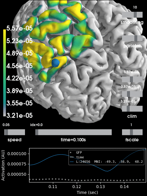
Alternatively, we can project the sensor data to the nearest locations on the pial surface and visualize that:
evoked = mne.EvokedArray(
gamma_power_t[:, sl], raw.info, tmin=raw.times[sl][0])
stc = mne.stc_near_sensors(evoked, trans, subject, subjects_dir=subjects_dir)
clim = dict(kind='value', lims=[vmin * 0.9, vmin, vmax])
brain = stc.plot(surface='pial', hemi='both', initial_time=0.68,
colormap='viridis', clim=clim, views='parietal',
subjects_dir=subjects_dir, size=(500, 500))
# You can save a movie like the one on our documentation website with:
# brain.save_movie(time_dilation=50, interpolation='linear', framerate=10,
# time_viewer=True)
Out:
Projecting data from 64 sensors onto 312273 surface vertices: sum mode
Projecting electrodes onto surface
Minimum projected intra-sensor distance: 5.1 mm
17761 / 312273 non-zero vertices
Total running time of the script: ( 0 minutes 52.725 seconds)
Estimated memory usage: 164 MB