Working with sEEG data¶

MNE supports working with more than just MEG and EEG data. Here we show some of the functions that can be used to facilitate working with stereoelectroencephalography (sEEG) data.

This example shows how to use:

sEEG data
channel locations in MNI space
projection into a volume

Note that our sample sEEG electrodes are already assumed to be in MNI space. If you want to map positions from your subject MRI space to MNI fsaverage space, you must apply the FreeSurfer’s talairach.xfm transform for your dataset. You can take a look at How MNE uses FreeSurfer’s outputs for more information.

For an example that involves ECoG data, channel locations in a subject-specific MRI, or projection into a surface, see Working with ECoG data. In the ECoG example, we show how to visualize surface grid channels on the brain.

# Authors: Eric Larson <larson.eric.d@gmail.com>
#          Adam Li <adam2392@gmail.com>
#
# License: BSD (3-clause)

import os.path as op

import numpy as np
import pandas as pd

import mne
from mne.datasets import fetch_fsaverage

print(__doc__)

# paths to mne datasets - sample sEEG and FreeSurfer's fsaverage subject
# which is in MNI space
misc_path = mne.datasets.misc.data_path()
sample_path = mne.datasets.sample.data_path()
subject = 'fsaverage'
subjects_dir = sample_path + '/subjects'

# use mne-python's fsaverage data
fetch_fsaverage(subjects_dir=subjects_dir, verbose=True)  # downloads if needed

Out:

0 files missing from /home/circleci/project/mne/datasets/_fsaverage/root.txt in /home/circleci/mne_data/MNE-sample-data/subjects
0 files missing from /home/circleci/project/mne/datasets/_fsaverage/bem.txt in /home/circleci/mne_data/MNE-sample-data/subjects/fsaverage

Let’s load some sEEG electrode locations and names, and turn them into a mne.channels.DigMontage class. First, use pandas to read in the .tsv file.

# In mne-python, the electrode coordinates are required to be in meters
elec_df = pd.read_csv(misc_path + '/seeg/sample_seeg_electrodes.tsv',
                      sep='\t', header=0, index_col=None)
ch_names = elec_df['name'].tolist()
ch_coords = elec_df[['x', 'y', 'z']].to_numpy(dtype=float)

# the test channel coordinates were in mm, so we convert them to meters
ch_coords = ch_coords / 1000.

# create dictionary of channels and their xyz coordinates (now in MNI space)
ch_pos = dict(zip(ch_names, ch_coords))

# Ideally the nasion/LPA/RPA will also be present from the digitization, here
# we use fiducials estimated from the subject's FreeSurfer MNI transformation:
lpa, nasion, rpa = mne.coreg.get_mni_fiducials(
    subject, subjects_dir=subjects_dir)
lpa, nasion, rpa = lpa['r'], nasion['r'], rpa['r']

Now we make a mne.channels.DigMontage stating that the sEEG contacts are in the FreeSurfer surface RAS (i.e., MRI) coordinate system for the given subject. Keep in mind that fsaverage is special in that it is already in MNI space.

montage = mne.channels.make_dig_montage(
    ch_pos, coord_frame='mri', nasion=nasion, lpa=lpa, rpa=rpa)
print('Created %s channel positions' % len(ch_names))

Out:

Created 88 channel positions

Now we get the trans that transforms from our MRI coordinate system to the head coordinate frame. This transform will be applied to the data when applying the montage so that standard plotting functions like mne.viz.plot_evoked_topomap() will be aligned properly.

trans = mne.channels.compute_native_head_t(montage)
print(trans)

Out:

<Transform | MRI (surface RAS)->head>
[[ 9.99993682e-01  3.55187384e-03  2.02048104e-04 -1.76272495e-03]
 [-3.55756865e-03  9.98389125e-01  5.66258579e-02  3.10943504e-02]
 [-5.94736775e-07 -5.66262193e-02  9.98395443e-01  3.95972491e-02]
 [ 0.00000000e+00  0.00000000e+00  0.00000000e+00  1.00000000e+00]]

Now that we have our montage, we can load in our corresponding time-series data and set the montage to the raw data.

# first we'll load in the sample dataset
raw = mne.io.read_raw_edf(misc_path + '/seeg/sample_seeg.edf')

# drop bad channels
raw.info['bads'].extend([ch for ch in raw.ch_names if ch not in ch_names])
raw.load_data()
raw.drop_channels(raw.info['bads'])
raw.crop(0, 2)  # just process 2 sec of data for speed

# attach montage
raw.set_montage(montage)

# set channel types to sEEG (instead of EEG) that have actual positions
raw.set_channel_types(
    {ch_name: 'seeg' if np.isfinite(ch_pos[ch_name]).all() else 'misc'
     for ch_name in raw.ch_names})

Out:

Extracting EDF parameters from /home/circleci/mne_data/MNE-misc-data/seeg/sample_seeg.edf...
EDF file detected
Setting channel info structure...
Creating raw.info structure...
Reading 0 ... 19999  =      0.000 ...    19.999 secs...

Let’s check to make sure everything is aligned.

fig = mne.viz.plot_alignment(raw.info, trans, 'fsaverage',
                             subjects_dir=subjects_dir, show_axes=True,
                             surfaces=["pial", "head"])

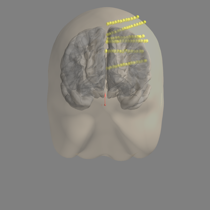
Out:

Using outer_skin.surf for head surface.
Plotting 88 sEEG locations

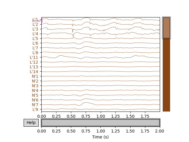
Next, we’ll get the raw data and plot its amplitude over time.

raw.plot()

We can visualize this raw data on the fsaverage brain (in MNI space) as a heatmap. This works by first creating an Evoked data structure from the data of interest (in this example, it is just the raw LFP). Then one should generate a stc data structure, which will be able to visualize source activity on the brain in various different formats.

# get standard fsaverage volume (5mm grid) source space
fname_src = op.join(subjects_dir, 'fsaverage', 'bem',
                    'fsaverage-vol-5-src.fif')
vol_src = mne.read_source_spaces(fname_src)

evoked = mne.EvokedArray(raw.get_data(), raw.info).crop(0, 1)  # shorter
stc = mne.stc_near_sensors(
    evoked, trans, subject, subjects_dir=subjects_dir, src=vol_src,
    verbose='error')  # ignore missing electrode warnings
stc = abs(stc)  # just look at magnitude
clim = dict(kind='value', lims=np.percentile(abs(evoked.data), [10, 50, 75]))

Out:

Reading a source space...
[done]
1 source spaces read

Plot 3D source (brain region) visualization:

By default, stc.plot_3d() will show a time course of the source with the largest absolute value across any time point. In this example, it is simply the source with the largest raw signal value. Its location is marked on the brain by a small blue sphere.

brain = stc.plot_3d(
    src=vol_src, subjects_dir=subjects_dir,
    view_layout='horizontal', views=['axial', 'coronal', 'sagittal'],
    size=(800, 300), show_traces=0.4, clim=clim,
    add_data_kwargs=dict(colorbar_kwargs=dict(label_font_size=8)))

# You can save a movie like the one on our documentation website with:
# brain.save_movie(time_dilation=3, interpolation='linear', framerate=10,
#                  time_viewer=True, filename='./mne-test-seeg.m4')

In this tutorial, we used a BEM surface for the fsaverage subject from FreeSurfer.

For additional common analyses of interest, see the following:

For volumetric plotting options, including limiting to a specific area of the volume specified by say an atlas, or plotting different types of source visualizations see: Visualize source time courses (stcs).
For extracting activation within a specific FreeSurfer volume and using different FreeSurfer volumes, see: How MNE uses FreeSurfer’s outputs.
For working with BEM surfaces and using FreeSurfer, or mne to generate them, see: Head model and forward computation.

Total running time of the script: ( 1 minutes 13.377 seconds)

Estimated memory usage: 563 MB