Modifying data in-place¶

It is often necessary to modify data once you have loaded it into memory. Common examples of this are signal processing, feature extraction, and data cleaning. Some functionality is pre-built into MNE-python, though it is also possible to apply an arbitrary function to the data.

import mne
import os.path as op
import numpy as np
from matplotlib import pyplot as plt

Load an example dataset, the preload flag loads the data into memory now

data_path = op.join(mne.datasets.sample.data_path(), 'MEG',
                    'sample', 'sample_audvis_raw.fif')
raw = mne.io.read_raw_fif(data_path, preload=True)
raw = raw.crop(0, 10)
print(raw)

Out:

Opening raw data file /home/circleci/mne_data/MNE-sample-data/MEG/sample/sample_audvis_raw.fif...
    Read a total of 3 projection items:
        PCA-v1 (1 x 102)  idle
        PCA-v2 (1 x 102)  idle
        PCA-v3 (1 x 102)  idle
    Range : 25800 ... 192599 =     42.956 ...   320.670 secs
Ready.
Reading 0 ... 166799  =      0.000 ...   277.714 secs...
<Raw | sample_audvis_raw.fif, 376 x 6007 (10.0 s), ~20.5 MB, data loaded>

Signal processing¶

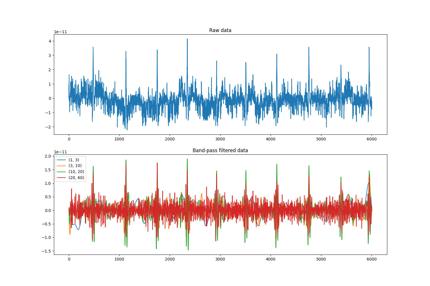
Most MNE objects have in-built methods for filtering:

filt_bands = [(1, 3), (3, 10), (10, 20), (20, 60)]
_, (ax, ax2) = plt.subplots(2, 1, figsize=(15, 10))
data, times = raw[0]
_ = ax.plot(data[0])
for fmin, fmax in filt_bands:
    raw_filt = raw.copy()
    raw_filt.filter(fmin, fmax, fir_design='firwin')
    _ = ax2.plot(raw_filt[0][0][0])
ax2.legend(filt_bands)
ax.set_title('Raw data')
ax2.set_title('Band-pass filtered data')

Out:

Filtering raw data in 1 contiguous segment
Setting up band-pass filter from 1 - 3 Hz

FIR filter parameters
---------------------
Designing a one-pass, zero-phase, non-causal bandpass filter:
- Windowed time-domain design (firwin) method
- Hamming window with 0.0194 passband ripple and 53 dB stopband attenuation
- Lower passband edge: 1.00
- Lower transition bandwidth: 1.00 Hz (-6 dB cutoff frequency: 0.50 Hz)
- Upper passband edge: 3.00 Hz
- Upper transition bandwidth: 2.00 Hz (-6 dB cutoff frequency: 4.00 Hz)
- Filter length: 1983 samples (3.302 sec)

Filtering raw data in 1 contiguous segment
Setting up band-pass filter from 3 - 10 Hz

FIR filter parameters
---------------------
Designing a one-pass, zero-phase, non-causal bandpass filter:
- Windowed time-domain design (firwin) method
- Hamming window with 0.0194 passband ripple and 53 dB stopband attenuation
- Lower passband edge: 3.00
- Lower transition bandwidth: 2.00 Hz (-6 dB cutoff frequency: 2.00 Hz)
- Upper passband edge: 10.00 Hz
- Upper transition bandwidth: 2.50 Hz (-6 dB cutoff frequency: 11.25 Hz)
- Filter length: 993 samples (1.653 sec)

Filtering raw data in 1 contiguous segment
Setting up band-pass filter from 10 - 20 Hz

FIR filter parameters
---------------------
Designing a one-pass, zero-phase, non-causal bandpass filter:
- Windowed time-domain design (firwin) method
- Hamming window with 0.0194 passband ripple and 53 dB stopband attenuation
- Lower passband edge: 10.00
- Lower transition bandwidth: 2.50 Hz (-6 dB cutoff frequency: 8.75 Hz)
- Upper passband edge: 20.00 Hz
- Upper transition bandwidth: 5.00 Hz (-6 dB cutoff frequency: 22.50 Hz)
- Filter length: 793 samples (1.320 sec)

Filtering raw data in 1 contiguous segment
Setting up band-pass filter from 20 - 60 Hz

FIR filter parameters
---------------------
Designing a one-pass, zero-phase, non-causal bandpass filter:
- Windowed time-domain design (firwin) method
- Hamming window with 0.0194 passband ripple and 53 dB stopband attenuation
- Lower passband edge: 20.00
- Lower transition bandwidth: 5.00 Hz (-6 dB cutoff frequency: 17.50 Hz)
- Upper passband edge: 60.00 Hz
- Upper transition bandwidth: 15.00 Hz (-6 dB cutoff frequency: 67.50 Hz)
- Filter length: 397 samples (0.661 sec)

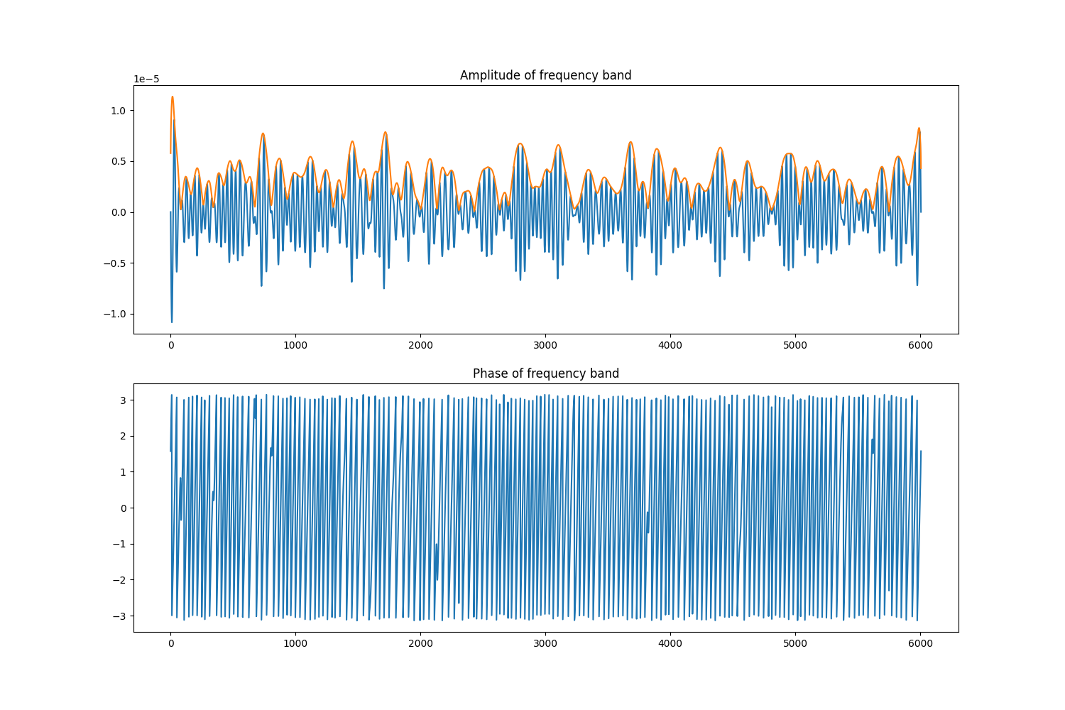
In addition, there are functions for applying the Hilbert transform, which is useful to calculate phase / amplitude of your signal.

# Filter signal with a fairly steep filter, then take hilbert transform

raw_band = raw.copy()
raw_band.filter(12, 18, l_trans_bandwidth=2., h_trans_bandwidth=2.,
                fir_design='firwin')
raw_hilb = raw_band.copy()
hilb_picks = mne.pick_types(raw_band.info, meg=False, eeg=True)
raw_hilb.apply_hilbert(hilb_picks)
print(raw_hilb[0][0].dtype)

Out:

Filtering raw data in 1 contiguous segment
Setting up band-pass filter from 12 - 18 Hz

FIR filter parameters
---------------------
Designing a one-pass, zero-phase, non-causal bandpass filter:
- Windowed time-domain design (firwin) method
- Hamming window with 0.0194 passband ripple and 53 dB stopband attenuation
- Lower passband edge: 12.00
- Lower transition bandwidth: 2.00 Hz (-6 dB cutoff frequency: 11.00 Hz)
- Upper passband edge: 18.00 Hz
- Upper transition bandwidth: 2.00 Hz (-6 dB cutoff frequency: 19.00 Hz)
- Filter length: 993 samples (1.653 sec)

complex128

Finally, it is possible to apply arbitrary functions to your data to do what you want. Here we will use this to take the amplitude and phase of the hilbert transformed data.

Note

You can also use envelope=True in the call to mne.io.Raw.apply_hilbert() to do this automatically.

# Take the amplitude and phase
raw_amp = raw_hilb.copy()
raw_amp.apply_function(np.abs, hilb_picks)
raw_phase = raw_hilb.copy()
raw_phase.apply_function(np.angle, hilb_picks)

_, (a1, a2) = plt.subplots(2, 1, figsize=(15, 10))
a1.plot(raw_band[hilb_picks[0]][0][0].real)
a1.plot(raw_amp[hilb_picks[0]][0][0].real)
a2.plot(raw_phase[hilb_picks[0]][0][0].real)
a1.set_title('Amplitude of frequency band')
a2.set_title('Phase of frequency band')