Annotating continuous data

This tutorial describes adding annotations to a Raw object, and how annotations are used in later stages of data processing.

As usual we’ll start by importing the modules we need, loading some example data, and (since we won’t actually analyze the raw data in this tutorial) cropping the Raw object to just 60 seconds before loading it into RAM to save memory:

import os
from datetime import timedelta
import mne

sample_data_folder = mne.datasets.sample.data_path()
sample_data_raw_file = os.path.join(sample_data_folder, 'MEG', 'sample',
                                    'sample_audvis_raw.fif')
raw = mne.io.read_raw_fif(sample_data_raw_file, verbose=False)
raw.crop(tmax=60).load_data()

Annotations in MNE-Python are a way of storing short strings of information about temporal spans of a Raw object. Below the surface, Annotations are list-like objects, where each element comprises three pieces of information: an onset time (in seconds), a duration (also in seconds), and a description (a text string). Additionally, the Annotations object itself also keeps track of orig_time, which is a POSIX timestamp denoting a real-world time relative to which the annotation onsets should be interpreted.

Creating annotations programmatically

If you know in advance what spans of the Raw object you want to annotate, Annotations can be created programmatically, and you can even pass lists or arrays to the Annotations constructor to annotate multiple spans at once:

my_annot = mne.Annotations(onset=[3, 5, 7],
                           duration=[1, 0.5, 0.25],
                           description=['AAA', 'BBB', 'CCC'])
print(my_annot)

Out:

<Annotations | 3 segments: AAA (1), BBB (1), CCC (1)>

Notice that orig_time is None, because we haven’t specified it. In those cases, when you add the annotations to a Raw object, it is assumed that the orig_time matches the time of the first sample of the recording, so orig_time will be set to match the recording measurement date (raw.info['meas_date']).

raw.set_annotations(my_annot)
print(raw.annotations)

# convert meas_date (a tuple of seconds, microseconds) into a float:
meas_date = raw.info['meas_date']
orig_time = raw.annotations.orig_time
print(meas_date == orig_time)

Out:

<Annotations | 3 segments: AAA (1), BBB (1), CCC (1)>
True

Since the example data comes from a Neuromag system that starts counting sample numbers before the recording begins, adding my_annot to the Raw object also involved another automatic change: an offset equalling the time of the first recorded sample (raw.first_samp / raw.info['sfreq']) was added to the onset values of each annotation (see Time, sample number, and sample index for more info on raw.first_samp):

time_of_first_sample = raw.first_samp / raw.info['sfreq']
print(my_annot.onset + time_of_first_sample)
print(raw.annotations.onset)

Out:

[45.95597083 47.95597083 49.95597083]
[45.95597083 47.95597083 49.95597083]

If you know that your annotation onsets are relative to some other time, you can set orig_time before you call set_annotations(), and the onset times will get adjusted based on the time difference between your specified orig_time and raw.info['meas_date'], but without the additional adjustment for raw.first_samp. orig_time can be specified in various ways (see the documentation of Annotations for the options); here we’ll use an ISO 8601 formatted string, and set it to be 50 seconds later than raw.info['meas_date'].

time_format = '%Y-%m-%d %H:%M:%S.%f'
new_orig_time = (meas_date + timedelta(seconds=50)).strftime(time_format)
print(new_orig_time)

later_annot = mne.Annotations(onset=[3, 5, 7],
                              duration=[1, 0.5, 0.25],
                              description=['DDD', 'EEE', 'FFF'],
                              orig_time=new_orig_time)

raw2 = raw.copy().set_annotations(later_annot)
print(later_annot.onset)
print(raw2.annotations.onset)

Out:

2002-12-03 19:02:00.720100
[3. 5. 7.]
[53. 55. 57.]

Note

If your annotations fall outside the range of data times in the Raw object, the annotations outside the data range will not be added to raw.annotations, and a warning will be issued.

Now that your annotations have been added to a Raw object, you can see them when you visualize the Raw object:

fig = raw.plot(start=2, duration=6)

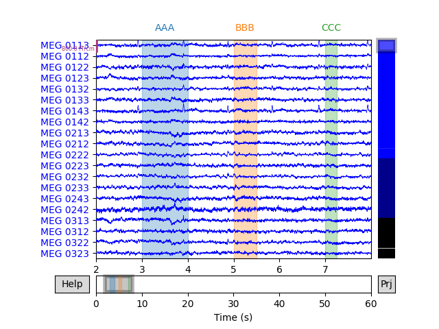
The three annotations appear as differently colored rectangles because they have different description values (which are printed along the top edge of the plot area). Notice also that colored spans appear in the small scroll bar at the bottom of the plot window, making it easy to quickly view where in a Raw object the annotations are so you can easily browse through the data to find and examine them.

Annotating Raw objects interactively

Annotations can also be added to a Raw object interactively by clicking-and-dragging the mouse in the plot window. To do this, you must first enter “annotation mode” by pressing a while the plot window is focused; this will bring up the annotation controls window:

fig.canvas.key_press_event('a')

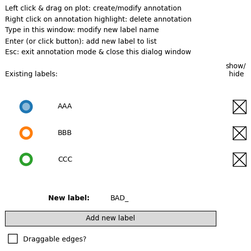
The colored rings are clickable, and determine which existing label will be created by the next click-and-drag operation in the main plot window. New annotation descriptions can be added by typing the new description, clicking the Add label button; the new description will be added to the list of descriptions and automatically selected.

During interactive annotation it is also possible to adjust the start and end times of existing annotations, by clicking-and-dragging on the left or right edges of the highlighting rectangle corresponding to that annotation.

Warning

Calling set_annotations() replaces any annotations currently stored in the Raw object, so be careful when working with annotations that were created interactively (you could lose a lot of work if you accidentally overwrite your interactive annotations). A good safeguard is to run interactive_annot = raw.annotations after you finish an interactive annotation session, so that the annotations are stored in a separate variable outside the Raw object.

How annotations affect preprocessing and analysis

You may have noticed that the description for new labels in the annotation controls window defaults to BAD_. The reason for this is that annotation is often used to mark bad temporal spans of data (such as movement artifacts or environmental interference that cannot be removed in other ways such as projection or filtering). Several MNE-Python operations are “annotation aware” and will avoid using data that is annotated with a description that begins with “bad” or “BAD”; such operations typically have a boolean reject_by_annotation parameter. Examples of such operations are independent components analysis (mne.preprocessing.ICA), functions for finding heartbeat and blink artifacts (find_ecg_events(), find_eog_events()), and creation of epoched data from continuous data (mne.Epochs). See Rejecting bad data spans for details.

Operations on Annotations objects

Annotations objects can be combined by simply adding them with the + operator, as long as they share the same orig_time:

new_annot = mne.Annotations(onset=3.75, duration=0.75, description='AAA')
raw.set_annotations(my_annot + new_annot)
raw.plot(start=2, duration=6)

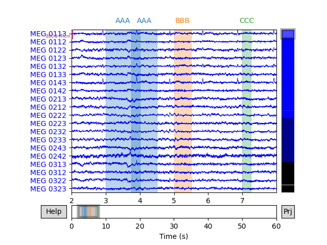
Notice that it is possible to create overlapping annotations, even when they share the same description. This is not possible when annotating interactively; click-and-dragging to create a new annotation that overlaps with an existing annotation with the same description will cause the old and new annotations to be merged.

Individual annotations can be accessed by indexing an Annotations object, and subsets of the annotations can be achieved by either slicing or indexing with a list, tuple, or array of indices:

print(raw.annotations[0])       # just the first annotation
print(raw.annotations[:2])      # the first two annotations
print(raw.annotations[(3, 2)])  # the fourth and third annotations

Out:

OrderedDict([('onset', 45.95597082905339), ('duration', 1.0), ('description', 'AAA'), ('orig_time', datetime.datetime(2002, 12, 3, 19, 1, 10, 720100, tzinfo=datetime.timezone.utc))])
<Annotations | 2 segments: AAA (2)>
<Annotations | 2 segments: BBB (1), CCC (1)>

You can also iterate over the annotations within an Annotations object:

for ann in raw.annotations:
    descr = ann['description']
    start = ann['onset']
    end = ann['onset'] + ann['duration']
    print("'{}' goes from {} to {}".format(descr, start, end))

Out:

'AAA' goes from 45.95597082905339 to 46.95597082905339
'AAA' goes from 46.70597082905339 to 47.45597082905339
'BBB' goes from 47.95597082905339 to 48.45597082905339
'CCC' goes from 49.95597082905339 to 50.20597082905339

Note that iterating, indexing and slicing Annotations all return a copy, so changes to an indexed, sliced, or iterated element will not modify the original Annotations object.

# later_annot WILL be changed, because we're modifying the first element of
# later_annot.onset directly:
later_annot.onset[0] = 99

# later_annot WILL NOT be changed, because later_annot[0] returns a copy
# before the 'onset' field is changed:
later_annot[0]['onset'] = 77

print(later_annot[0]['onset'])

Out:

99.0

Reading and writing Annotations to/from a file

Annotations objects have a save() method which can write .fif, .csv, and .txt formats (the format to write is inferred from the file extension in the filename you provide). There is a corresponding read_annotations() function to load them from disk:

raw.annotations.save('saved-annotations.csv')
annot_from_file = mne.read_annotations('saved-annotations.csv')
print(annot_from_file)

Out:

<Annotations | 4 segments: AAA (2), BBB (1), CCC (1)>

Estimated memory usage: 221 MB