How MNE uses FreeSurfer’s outputs

This tutorial explains how MRI coordinate frames are handled in MNE-Python, and how MNE-Python integrates with FreeSurfer for handling MRI data and source space data in general.

As usual we’ll start by importing the necessary packages; for this tutorial that includes nibabel to handle loading the MRI images (MNE-Python also uses nibabel under the hood). We’ll also use a special Matplotlib function for adding outlines to text, so that text is readable on top of an MRI image.

import os

import numpy as np
import nibabel
import matplotlib.pyplot as plt
import matplotlib.patheffects as path_effects

import mne
from mne.transforms import apply_trans
from mne.io.constants import FIFF

MRI coordinate frames

Let’s start out by looking at the sample subject MRI. Following standard FreeSurfer convention, we look at T1.mgz, which gets created from the original MRI sample/mri/orig/001.mgz when you run the FreeSurfer command recon-all. Here we use nibabel to load the T1 image, and the resulting object’s orthoview() method to view it.

data_path = mne.datasets.sample.data_path()
subjects_dir = os.path.join(data_path, 'subjects')
subject = 'sample'
t1_fname = os.path.join(subjects_dir, subject, 'mri', 'T1.mgz')
t1 = nibabel.load(t1_fname)
t1.orthoview()

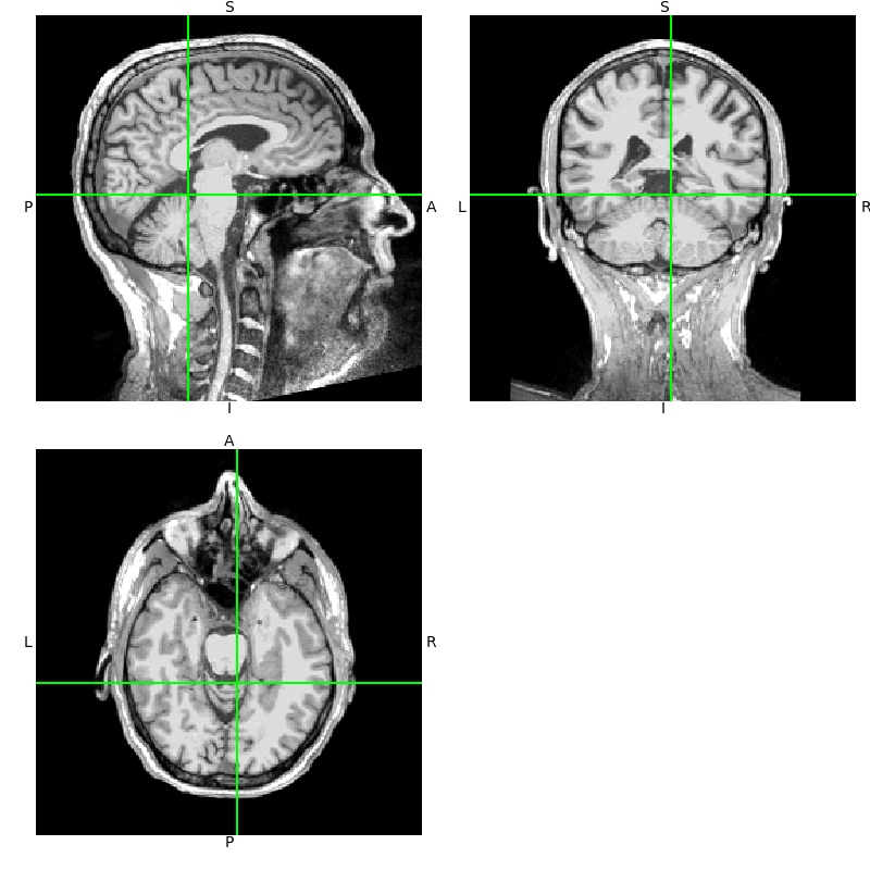
Notice that the axes in the orthoview() figure are labeled L-R, S-I, and P-A. These reflect the standard RAS (right-anterior-superior) coordinate system that is widely used in MRI imaging. If you are unfamiliar with RAS coordinates, see the excellent nibabel tutorial Coordinate systems and affines.

Nibabel already takes care of some coordinate frame transformations under the hood, so let’s do it manually so we understand what is happening. First let’s get our data as a 3D array and note that it’s already a standard size:

data = np.asarray(t1.dataobj)
print(data.shape)

Out:

(256, 256, 256)

These data are voxel intensity values. Here they are unsigned integers in the range 0-255, though in general they can be floating point values. A value data[i, j, k] at a given index triplet (i, j, k) corresponds to some real-world physical location (x, y, z) in space. To get its physical location, first we have to choose what coordinate frame we’re going to use.

For example, we could choose a geographical coordinate frame, with origin is at the center of the earth, Z axis through the north pole, X axis through the prime meridian (zero degrees longitude), and Y axis orthogonal to these forming a right-handed coordinate system. This would not be a very useful choice for defining the physical locations of the voxels during the MRI acquisition for analysis, but you could nonetheless figure out the transformation that related the (i, j, k) to this coordinate frame.

Instead, each scanner defines a more practical, native coordinate system that it uses during acquisition, usually related to the physical orientation of the scanner itself and/or the subject within it. During acquisition the relationship between the voxel indices (i, j, k) and the physical location (x, y, z) in the scanner’s native coordinate frame is saved in the image’s affine transformation.

Under the hood

mne.transforms.apply_trans effectively does a matrix multiplication (i.e., numpy.dot()), with a little extra work to handle the shape mismatch (the affine has shape (4, 4) because it includes a translation, which is applied separately).

We can use nibabel to examine this transformation, keeping in mind that it processes everything in units of millimeters, unlike MNE where things are always in SI units (meters).

This allows us to take an arbitrary voxel or slice of data and know where it is in the scanner’s native physical space (x, y, z) (in mm) by applying the affine transformation to the voxel coordinates.

print(t1.affine)
vox = np.array([122, 119, 102])
xyz_ras = apply_trans(t1.affine, vox)
print('Our voxel has real-world coordinates {}, {}, {} (mm)'
      .format(*np.round(xyz_ras, 3)))

Out:

[[-1.00000000e+00  1.15484021e-07 -1.91852465e-07  1.22726395e+02]
 [ 8.56816911e-08  1.57160827e-08  1.00000000e+00 -1.18960930e+02]
 [ 1.49011647e-08 -1.00000000e+00  6.40284092e-09  1.00712036e+02]
 [ 0.00000000e+00  0.00000000e+00  0.00000000e+00  1.00000000e+00]]
Our voxel has real-world coordinates 0.726, -16.961, -18.288 (mm)

If you have a point (x, y, z) in scanner-native RAS space and you want the corresponding voxel number, you can get it using the inverse of the affine. This involves some rounding, so it’s possible to end up off by one voxel if you’re not careful:

ras_coords_mm = np.array([1, -17, -18])
inv_affine = np.linalg.inv(t1.affine)
i_, j_, k_ = np.round(apply_trans(inv_affine, ras_coords_mm)).astype(int)
print('Our real-world coordinates correspond to voxel ({}, {}, {})'
      .format(i_, j_, k_))

Out:

Our real-world coordinates correspond to voxel (122, 119, 102)

Let’s write a short function to visualize where our voxel lies in an image, and annotate it in RAS space (rounded to the nearest millimeter):

def imshow_mri(data, img, vox, xyz, suptitle):
    """Show an MRI slice with a voxel annotated."""
    i, j, k = vox
    fig, ax = plt.subplots(1, figsize=(6, 6))
    codes = nibabel.orientations.aff2axcodes(img.affine)
    # Figure out the title based on the code of this axis
    ori_slice = dict(P='Coronal', A='Coronal',
                     I='Axial', S='Axial',
                     L='Sagittal', R='Saggital')
    ori_names = dict(P='posterior', A='anterior',
                     I='inferior', S='superior',
                     L='left', R='right')
    title = ori_slice[codes[0]]
    ax.imshow(data[i], vmin=10, vmax=120, cmap='gray', origin='lower')
    ax.axvline(k, color='y')
    ax.axhline(j, color='y')
    for kind, coords in xyz.items():
        annotation = ('{}: {}, {}, {} mm'
                      .format(kind, *np.round(coords).astype(int)))
        text = ax.text(k, j, annotation, va='baseline', ha='right',
                       color=(1, 1, 0.7))
        text.set_path_effects([
            path_effects.Stroke(linewidth=2, foreground='black'),
            path_effects.Normal()])
    # reorient view so that RAS is always rightward and upward
    x_order = -1 if codes[2] in 'LIP' else 1
    y_order = -1 if codes[1] in 'LIP' else 1
    ax.set(xlim=[0, data.shape[2] - 1][::x_order],
           ylim=[0, data.shape[1] - 1][::y_order],
           xlabel=f'k ({ori_names[codes[2]]}+)',
           ylabel=f'j ({ori_names[codes[1]]}+)',
           title=f'{title} view: i={i} ({ori_names[codes[0]]}+)')
    fig.suptitle(suptitle)
    fig.subplots_adjust(0.1, 0.1, 0.95, 0.85)
    return fig


imshow_mri(data, t1, vox, {'Scanner RAS': xyz_ras}, 'MRI slice')

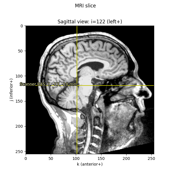
Notice that the axis scales (i, j, and k) are still in voxels (ranging from 0-255); it’s only the annotation text that we’ve translated into real-world RAS in millimeters.

“MRI coordinates” in MNE-Python: FreeSurfer surface RAS

While nibabel uses scanner RAS (x, y, z) coordinates, FreeSurfer uses a slightly different coordinate frame: MRI surface RAS. The transform from voxels to the FreeSurfer MRI surface RAS coordinate frame is known in the FreeSurfer documentation as Torig, and in nibabel as vox2ras_tkr. This transformation sets the center of its coordinate frame in the middle of the conformed volume dimensions (N / 2.) with the axes oriented along the axes of the volume itself. For more information, see MEG/EEG and MRI coordinate systems.

Note

In general, you should assume that the MRI coordinate system for a given subject is specific to that subject, i.e., it is not the same coordinate MRI coordinate system that is used for any other FreeSurfer subject. Even though during processing FreeSurfer will align each subject’s MRI to fsaverage to do reconstruction, all data (surfaces, MRIs, etc.) get stored in the coordinate frame specific to that subject. This is why it’s important for group analyses to transform data to a common coordinate frame for example by surface or volumetric morphing, or even by just applying FreeSurfer’s MNI affine transformation to points.

Since MNE-Python uses FreeSurfer extensively for surface computations (e.g., white matter, inner/outer skull meshes), internally MNE-Python uses the Freeurfer surface RAS coordinate system (not the nibabel scanner RAS system) for as many computations as possible, such as all source space and BEM mesh vertex definitions.

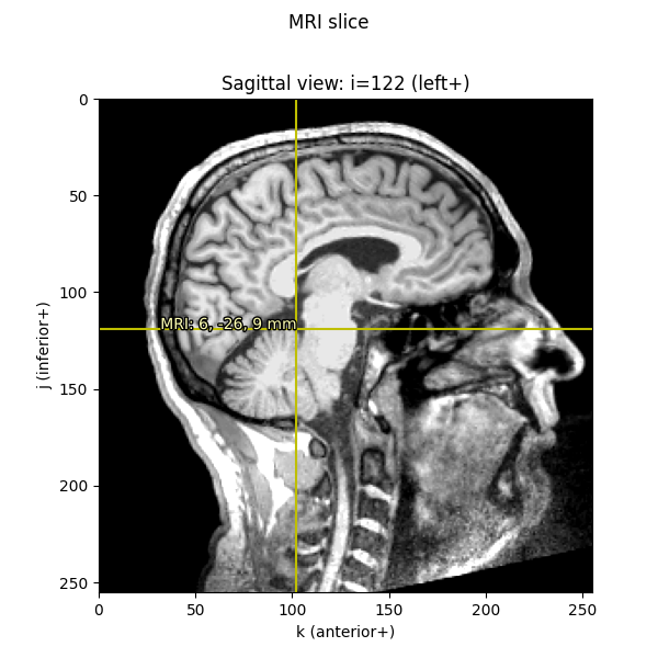
Whenever you see “MRI coordinates” or “MRI coords” in MNE-Python’s documentation, you should assume that we are talking about the “FreeSurfer MRI surface RAS” coordinate frame!

We can do similar computations as before to convert the given voxel indices into FreeSurfer MRI coordinates (i.e., what we call “MRI coordinates” or “surface RAS” everywhere else in MNE), just like we did above to convert voxel indices to scanner RAS:

Torig = t1.header.get_vox2ras_tkr()
print(t1.affine)
print(Torig)
xyz_mri = apply_trans(Torig, vox)
imshow_mri(data, t1, vox, dict(MRI=xyz_mri), 'MRI slice')

Out:

[[-1.00000000e+00  1.15484021e-07 -1.91852465e-07  1.22726395e+02]
 [ 8.56816911e-08  1.57160827e-08  1.00000000e+00 -1.18960930e+02]
 [ 1.49011647e-08 -1.00000000e+00  6.40284092e-09  1.00712036e+02]
 [ 0.00000000e+00  0.00000000e+00  0.00000000e+00  1.00000000e+00]]
[[  -1.    0.    0.  128.]
 [   0.    0.    1. -128.]
 [   0.   -1.    0.  128.]
 [   0.    0.    0.    1.]]

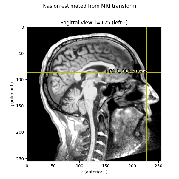
Knowing these relationships and being mindful about transformations, we can get from a point in any given space to any other space. Let’s start out by plotting the Nasion on a saggital MRI slice:

fiducials = mne.coreg.get_mni_fiducials(subject, subjects_dir=subjects_dir)
nasion_mri = [d for d in fiducials if d['ident'] == FIFF.FIFFV_POINT_NASION][0]
print(nasion_mri)  # note it's in Freesurfer MRI coords

Out:

<DigPoint |     Nasion : (2.6, 99.8, 40.8) mm      : MRI (surface RAS) frame>

When we print the nasion, it displays as a DigPoint and shows its coordinates in millimeters, but beware that the underlying data is actually stored in meters, so before transforming and plotting we’ll convert to millimeters:

nasion_mri = nasion_mri['r'] * 1000  # meters → millimeters
nasion_vox = np.round(
    apply_trans(np.linalg.inv(Torig), nasion_mri)).astype(int)
imshow_mri(data, t1, nasion_vox, dict(MRI=nasion_mri),
           'Nasion estimated from MRI transform')

We can also take the digitization point from the MEG data, which is in the “head” coordinate frame.

Let’s look at the nasion in the head coordinate frame:

info = mne.io.read_info(
    os.path.join(data_path, 'MEG', 'sample', 'sample_audvis_raw.fif'))
nasion_head = [d for d in info['dig'] if
               d['kind'] == FIFF.FIFFV_POINT_CARDINAL and
               d['ident'] == FIFF.FIFFV_POINT_NASION][0]
print(nasion_head)  # note it's in "head" coordinates

Out:

    Read a total of 3 projection items:
        PCA-v1 (1 x 102)  idle
        PCA-v2 (1 x 102)  idle
        PCA-v3 (1 x 102)  idle
<DigPoint |     Nasion : (0.0, 102.6, 0.0) mm      : head frame>

Head coordinate frame

The head coordinate frame in MNE is the “Neuromag” head coordinate frame. The origin is given by the intersection between a line connecting the LPA and RPA and the line orthogonal to it that runs through the nasion. It is also in RAS orientation, meaning that +X runs through the RPA, +Y goes through the nasion, and +Z is orthogonal to these pointing upward. See MEG/EEG and MRI coordinate systems for more information.

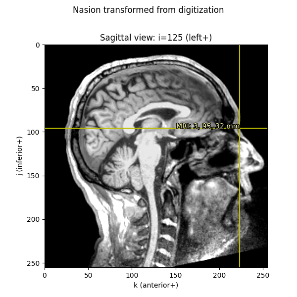
Notice that in “head” coordinate frame the nasion has values of 0 for the x and z directions (which makes sense given that the nasion is used to define the y axis in that system). To convert from head coordinate frame to voxels, we first apply the head → MRI (surface RAS) transform from a trans file (typically created with the MNE-Python coregistration GUI), then convert meters → millimeters, and finally apply the inverse of Torig to get to voxels.

Under the hood, functions like mne.setup_source_space(), mne.setup_volume_source_space(), and mne.compute_source_morph() make extensive use of these coordinate frames.

trans = mne.read_trans(
    os.path.join(data_path, 'MEG', 'sample', 'sample_audvis_raw-trans.fif'))

# first we transform from head to MRI, and *then* convert to millimeters
nasion_dig_mri = apply_trans(trans, nasion_head['r']) * 1000

# ...then we can use Torig to convert MRI to voxels:
nasion_dig_vox = np.round(
    apply_trans(np.linalg.inv(Torig), nasion_dig_mri)).astype(int)
imshow_mri(data, t1, nasion_dig_vox, dict(MRI=nasion_dig_mri),
           'Nasion transformed from digitization')

Using FreeSurfer’s surface reconstructions

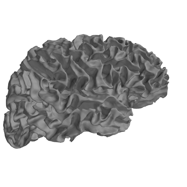
An important part of what FreeSurfer does is provide cortical surface reconstructions. For example, let’s load and view the white surface of the brain. This is a 3D mesh defined by a set of vertices (conventionally called rr) with shape (n_vertices, 3) and a set of triangles (tris) with shape (n_tris, 3) defining which vertices in rr form each triangular facet of the mesh.

fname = os.path.join(subjects_dir, subject, 'surf', 'rh.white')
rr_mm, tris = mne.read_surface(fname)
print(f'rr_mm.shape == {rr_mm.shape}')
print(f'tris.shape == {tris.shape}')
print(f'rr_mm.max() = {rr_mm.max()}')  # just to show that we are in mm

Out:

rr_mm.shape == (156866, 3)
tris.shape == (313728, 3)
rr_mm.max() = 97.80481719970703

Let’s actually plot it:

renderer = mne.viz.backends.renderer.create_3d_figure(
    size=(600, 600), bgcolor='w', scene=False)
gray = (0.5, 0.5, 0.5)
renderer.mesh(*rr_mm.T, triangles=tris, color=gray)
view_kwargs = dict(elevation=90, azimuth=0)
mne.viz.set_3d_view(
    figure=renderer.figure, distance=350, focalpoint=(0., 0., 40.),
    **view_kwargs)
renderer.show()

We can also plot the mesh on top of an MRI slice. The mesh surfaces are defined in millimeters in the MRI (FreeSurfer surface RAS) coordinate frame, so we can convert them to voxels by applying the inverse of the Torig transform:

rr_vox = apply_trans(np.linalg.inv(Torig), rr_mm)
fig = imshow_mri(data, t1, vox, {'Scanner RAS': xyz_ras}, 'MRI slice')
# Based on how imshow_mri works, the "X" here is the last dim of the MRI vol,
# the "Y" is the middle dim, and the "Z" is the first dim, so now that our
# points are in the correct coordinate frame, we need to ask matplotlib to
# do a tricontour slice like:
fig.axes[0].tricontour(rr_vox[:, 2], rr_vox[:, 1], tris, rr_vox[:, 0],
                       levels=[vox[0]], colors='r', linewidths=1.0,
                       zorder=1)

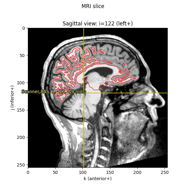
This is the method used by mne.viz.plot_bem() to show the BEM surfaces.

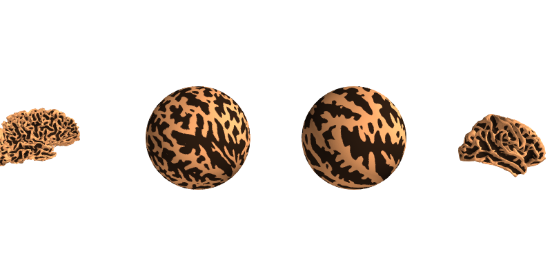
Cortical alignment (spherical)

A critical function provided by FreeSurfer is spherical surface alignment of cortical surfaces, maximizing sulcal-gyral alignment. FreeSurfer first expands the cortical surface to a sphere, then aligns it optimally with fsaverage. Because the vertex ordering is preserved when expanding to a sphere, a given vertex in the source (sample) mesh can be mapped easily to the same location in the destination (fsaverage) mesh, and vice-versa.

renderer_kwargs = dict(bgcolor='w', smooth_shading=False)
renderer = mne.viz.backends.renderer.create_3d_figure(
    size=(800, 400), scene=False, **renderer_kwargs)
curvs = [
    (mne.surface.read_curvature(os.path.join(
        subjects_dir, subj, 'surf', 'rh.curv'),
        binary=False) > 0).astype(float)
    for subj in ('sample', 'fsaverage') for _ in range(2)]
fnames = [os.path.join(subjects_dir, subj, 'surf', surf)
          for subj in ('sample', 'fsaverage')
          for surf in ('rh.white', 'rh.sphere')]
y_shifts = [-450, -150, 450, 150]
z_shifts = [-40, 0, -30, 0]
for name, y_shift, z_shift, curv in zip(fnames, y_shifts, z_shifts, curvs):
    this_rr, this_tri = mne.read_surface(name)
    this_rr += [0, y_shift, z_shift]
    renderer.mesh(*this_rr.T, triangles=this_tri, color=None, scalars=curv,
                  colormap='copper_r', vmin=-0.2, vmax=1.2)
zero = [0., 0., 0.]
width = 50.
y = np.sort(y_shifts)
y = (y[1:] + y[:-1]) / 2. - width / 2.
renderer.quiver3d(zero, y, zero,
                  zero, [1] * 3, zero, 'k', width, 'arrow')
view_kwargs['focalpoint'] = (0., 0., 0.)
mne.viz.set_3d_view(figure=renderer.figure, distance=1000, **view_kwargs)
renderer.show()

Let’s look a bit more closely at the spherical alignment by overlaying the two spherical meshes as wireframes and zooming way in (the purple points are separated by about 1 mm):

cyan = '#66CCEE'
purple = '#AA3377'
renderer = mne.viz.backends.renderer.create_3d_figure(
    size=(800, 800), scene=False, **renderer_kwargs)
fnames = [os.path.join(subjects_dir, subj, 'surf', 'rh.sphere')
          for subj in ('sample', 'fsaverage')]
colors = [cyan, purple]
for name, color in zip(fnames, colors):
    this_rr, this_tri = mne.read_surface(name)
    renderer.mesh(*this_rr.T, triangles=this_tri, color=color,
                  representation='wireframe')
mne.viz.set_3d_view(figure=renderer.figure, distance=20, **view_kwargs)
renderer.show()

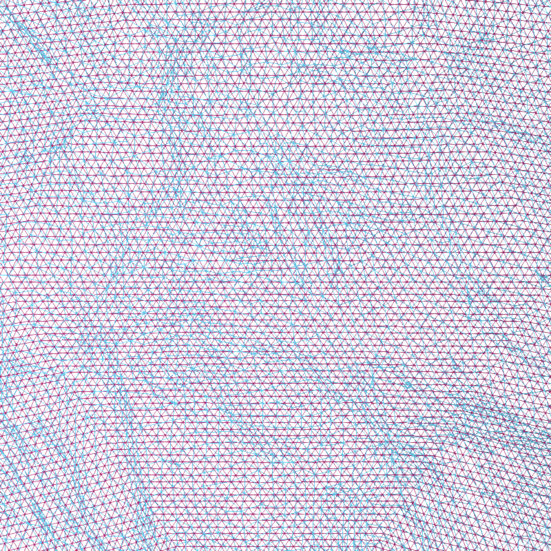
You can see that the fsaverage (purple) mesh is uniformly spaced, and the mesh for subject “sample” (in cyan) has been deformed along the spherical surface by FreeSurfer. This deformation is designed to optimize the sulcal-gyral alignment.

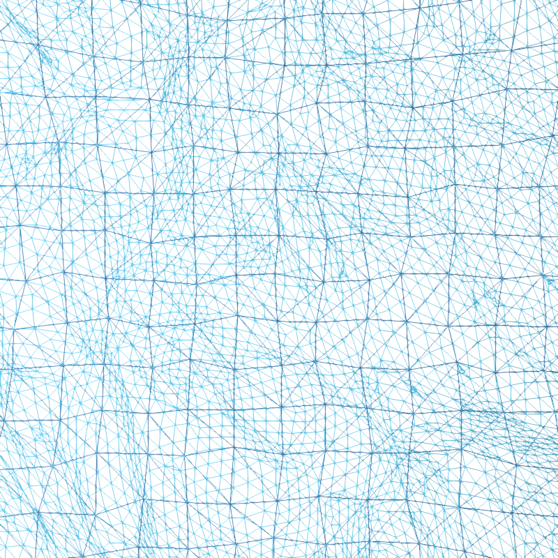
Surface decimation

These surfaces have a lot of vertices, and in general we only need to use a subset of these vertices for creating source spaces. A uniform sampling can easily be achieved by subsampling in the spherical space. To do this, we use a recursively subdivided icosahedron or octahedron. For example, let’s load a standard oct-6 source space, and at the same zoom level as before visualize how it subsampled the dense mesh:

src = mne.read_source_spaces(os.path.join(subjects_dir, 'sample', 'bem',
                                          'sample-oct-6-src.fif'))
print(src)

blue = '#4477AA'
renderer = mne.viz.backends.renderer.create_3d_figure(
    size=(800, 800), scene=False, **renderer_kwargs)
rr_sph, _ = mne.read_surface(fnames[0])
for tris, color in [(src[1]['tris'], cyan), (src[1]['use_tris'], blue)]:
    renderer.mesh(*rr_sph.T, triangles=tris, color=color,
                  representation='wireframe')
mne.viz.set_3d_view(figure=renderer.figure, distance=20, **view_kwargs)
renderer.show()

Out:

    Reading a source space...
    Computing patch statistics...
    Patch information added...
    Distance information added...
    [done]
    Reading a source space...
    Computing patch statistics...
    Patch information added...
    Distance information added...
    [done]
    2 source spaces read
<SourceSpaces: [<surface (lh), n_vertices=155407, n_used=4098>, <surface (rh), n_vertices=156866, n_used=4098>] MRI (surface RAS) coords, subject 'sample', ~27.4 MB>

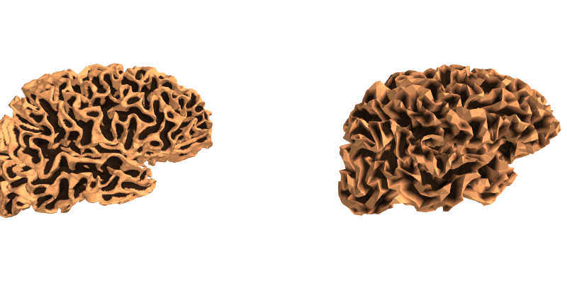
We can also then look at how these two meshes compare by plotting the original, high-density mesh as well as our decimated mesh white surfaces.

renderer = mne.viz.backends.renderer.create_3d_figure(
    size=(800, 400), scene=False, **renderer_kwargs)
y_shifts = [-125, 125]
tris = [src[1]['tris'], src[1]['use_tris']]
for y_shift, tris in zip(y_shifts, tris):
    this_rr = src[1]['rr'] * 1000. + [0, y_shift, -40]
    renderer.mesh(*this_rr.T, triangles=tris, color=None, scalars=curvs[0],
                  colormap='copper_r', vmin=-0.2, vmax=1.2)
renderer.quiver3d([0], [-width / 2.], [0], [0], [1], [0], 'k', width, 'arrow')
mne.viz.set_3d_view(figure=renderer.figure, distance=400, **view_kwargs)
renderer.show()

Warning

Some source space vertices can be removed during forward computation. See Head model and forward computation for more information.

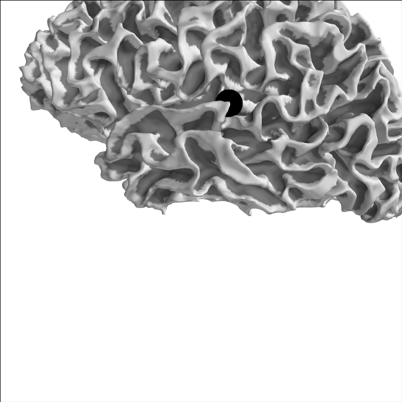
FreeSurfer’s MNI affine transformation

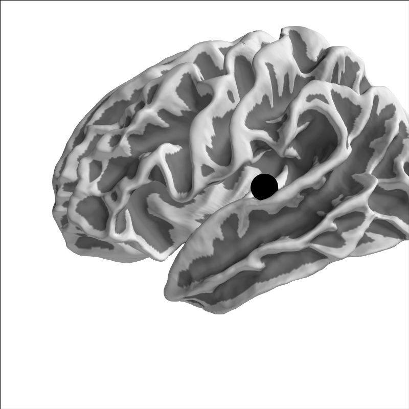
In addition to surface-based approaches, FreeSurfer also provides a simple affine coregistration of each subject’s data to the fsaverage subject. Let’s pick a point for sample and plot it on the brain:

brain = mne.viz.Brain('sample', 'lh', 'white', subjects_dir=subjects_dir,
                      background='w')
xyz = np.array([[-55, -10, 35]])
brain.add_foci(xyz, hemi='lh', color='k')
brain.show_view('lat')

We can take this point and transform it to MNI space:

mri_mni_trans = mne.read_talxfm(subject, subjects_dir)
print(mri_mni_trans)
xyz_mni = apply_trans(mri_mni_trans, xyz / 1000.) * 1000.
print(np.round(xyz_mni, 1))

Out:

<Transform | MRI (surface RAS)->MNI Talairach>
[[ 1.02248488 -0.00844919 -0.03621711  0.00111715]
 [ 0.07107091  0.91486582  0.40609791 -0.02300193]
 [ 0.00875602 -0.43369992  1.02811882 -0.03356932]
 [ 0.          0.          0.          1.        ]]
[[-56.3 -21.8   6.3]]

And because fsaverage is special in that it’s already in MNI space (its MRI-to-MNI transform is identity), it should land in the equivalent anatomical location:

brain = mne.viz.Brain('fsaverage', 'lh', 'white', subjects_dir=subjects_dir,
                      background='w')
brain.add_foci(xyz_mni, hemi='lh', color='k')
brain.show_view('lat')

Estimated memory usage: 26 MB