Algorithms and other implementation details

This page describes some of the technical details of MNE-Python implementation.

Internal representation (units)

Irrespective of the units used in your manufacturer’s format, when importing data, MNE-Python will always convert measurements to the same standard units. Thus the in-memory representation of data are always in:

• Volts (eeg, eog, seeg, emg, ecg, bio, ecog)

• Teslas (magnetometers)

• Teslas/meter (gradiometers)

• Amperes*meter (dipole fits, minimum-norm estimates, etc.)

• Moles/liter (“molar”; fNIRS data: oxyhemoglobin (hbo), deoxyhemoglobin (hbr))

• Arbitrary units (various derived unitless quantities)

Note, however, that most MNE-Python plotting functions will scale the data when plotted to yield nice-looking axis annotations in a sensible range; for example, mne.io.Raw.plot_psd() will convert teslas to femtoteslas (fT) and volts to microvolts (µV) when plotting MEG and EEG data.

The units used in internal data representation are particularly important to remember when extracting data from MNE-Python objects and manipulating it outside MNE-Python (e.g., when using methods like get_data() or to_data_frame() to convert data to NumPy arrays or Pandas DataFrames for analysis or plotting with other Python modules).

Floating-point precision

MNE-Python performs all computation in memory using the double-precision 64-bit floating point format. This means that the data is typecast into float64 format as soon as it is read into memory. The reason for this is that operations such as filtering and preprocessing are more accurate when using the 64-bit format. However, for backward compatibility, MNE-Python writes .fif files in a 32-bit format by default. This reduces file size when saving data to disk, but beware that saving intermediate results to disk and re-loading them from disk later may lead to loss in precision. If you would like to ensure 64-bit precision, there are two possibilities:

• Chain the operations in memory and avoid saving intermediate results.

• Save intermediate results but change the dtype used for saving, by using the fmt parameter of mne.io.Raw.save() (or mne.Epochs.save(), etc). However, note that this may render the .fif files unreadable in software packages other than MNE-Python.

Supported channel types

Channel types are represented in MNE-Python with shortened or abbreviated names. This page lists all supported channel types, their abbreviated names, and the measurement unit used to represent data of that type. Where channel types occur in two or more sub-types, the sub-type abbreviations are given in parentheses. More information about measurement units is given in the Internal representation (units) section.

Channel type	Description	Measurement unit
eeg	scalp electroencephalography (EEG)	Volts
meg (mag)	Magnetoencephalography (magnetometers)	Teslas
meg (grad)	Magnetoencephalography (gradiometers)	Teslas/meter
ecg	Electrocardiography (ECG)	Volts
seeg	Stereotactic EEG channels	Volts
ecog	Electrocorticography (ECoG)	Volts
fnirs (hbo)	Functional near-infrared spectroscopy (oxyhemoglobin)	Moles/liter
fnirs (hbr)	Functional near-infrared spectroscopy (deoxyhemoglobin)	Moles/liter
emg	Electromyography (EMG)	Volts
bio	Miscellaneous biological channels (e.g., skin conductance)	Arbitrary units
stim	stimulus (a.k.a. trigger) channels	Arbitrary units
resp	response-trigger channel	Arbitrary units
chpi	continuous head position indicator (HPI) coil channels	Teslas
exci	Flux excitation channel
ias	Internal Active Shielding data (Triux systems only?)
syst	System status channel information (Triux systems only)

Supported data formats

When MNE-Python loads sensor data, the data are stored in a Python object of type mne.io.Raw. Specialized loading functions are provided for the raw data file formats from a variety of equipment manufacturers. All raw data input/output functions in MNE-Python are found in mne.io and start with read_raw_*; see the documentation for each reader function for more info on reading specific file types.

As seen in the table below, there are also a few formats defined by other neuroimaging analysis software packages that are supported (EEGLAB, FieldTrip). Like the equipment-specific loading functions, these will also return an object of class Raw; additional functions are available for reading data that has already been epoched or averaged (see table).

Data type	File format	Extension	MNE-Python function
MEG	Artemis123	.bin	mne.io.read_raw_artemis123()
MEG	4-D Neuroimaging / BTi	<dir>	mne.io.read_raw_bti()
MEG	CTF	<dir>	mne.io.read_raw_ctf()
MEG and EEG	Elekta Neuromag	.fif	mne.io.read_raw_fif()
MEG	KIT	.sqd	mne.io.read_raw_kit(), mne.read_epochs_kit()
MEG and EEG	FieldTrip	.mat	mne.io.read_raw_fieldtrip(), mne.read_epochs_fieldtrip(), mne.read_evoked_fieldtrip()
EEG	Brainvision	.vhdr	mne.io.read_raw_brainvision()
EEG	Biosemi data format	.bdf	mne.io.read_raw_bdf()
EEG	Neuroscan CNT	.cnt	mne.io.read_raw_cnt()
EEG	European data format	.edf	mne.io.read_raw_edf()
EEG	EEGLAB	.set	mne.io.read_raw_eeglab(), mne.read_epochs_eeglab()
EEG	EGI simple binary	.egi	mne.io.read_raw_egi()
EEG	EGI MFF format	.mff	mne.io.read_raw_egi()
EEG	eXimia	.nxe	mne.io.read_raw_eximia()
EEG	General data format	.gdf	mne.io.read_raw_gdf()
EEG	Nicolet	.data	mne.io.read_raw_nicolet()
EEG	Persyst	.lay	mne.io.read_raw_persyst()
NIRS	NIRx	directory	mne.io.read_raw_nirx()
NIRS	BOXY	directory	mne.io.read_raw_boxy()

More details are provided in the tutorials in the Reading data for different recording systems section.

Supported formats for digitized 3D locations

MNE-Python can load 3D point locations obtained by digitization systems. Such files allow to obtain a montage that can then be added to Raw objects with the set_montage(). See the documentation for each reader function for more info on reading specific file types.

Vendor	Extension(s)	MNE-Python function
Neuromag	.fif	mne.channels.read_dig_fif()
Polhemus ISOTRAK	.hsp, .elp, .eeg	mne.channels.read_dig_polhemus_isotrak()
EGI	.xml	mne.channels.read_dig_egi()
MNE-C	.hpts	mne.channels.read_dig_hpts()
Brain Products	.bvct	mne.channels.read_dig_captrak()
Compumedics	.dat	mne.channels.read_dig_dat()

To load Polhemus FastSCAN files you can use montage.

It is also possible to make a montage from arrays with mne.channels.make_dig_montage().

Memory-efficient I/O

Preloading continuous (raw) data

MNE-Python can read data on-demand using the preload option provided in raw reading functions. For example:

from mne import io
from mne.datasets import sample
data_path = sample.data_path()
raw_fname = data_path + '/MEG/sample/sample_audvis_filt-0-40_raw.fif'
raw = io.read_raw_fif(raw_fname, preload=False)

Note

Filtering, resampling and dropping or selecting channels does not work with preload=False.

Preloading epoched data

Similarly, epochs can also be be read from disk on-demand. For example:

import mne
events = mne.find_events(raw)
event_id, tmin, tmax = 1, -0.2, 0.5
picks = mne.pick_types(raw.info, meg=True, eeg=True, stim=False, eog=True)
epochs = mne.Epochs(raw, events, event_id, tmin, tmax, picks=picks,
                    baseline=(None, 0), reject=dict(eeg=80e-6, eog=150e-6),
                    preload=False)

When preload=False, the epochs data is loaded from the disk on-demand. Note that preload=False for epochs will work even if the raw object has been loaded with preload=True. Preloading is also supported for mne.read_epochs().

Warning

This comes with a caveat. When preload=False, data rejection based on peak-to-peak thresholds is executed when the data is loaded from disk, not when the Epochs object is created.

To explicitly reject artifacts with preload=False, use the function mne.Epochs.drop_bad().

Loading data explicitly

To load the data if preload=False was initially selected, use the functions mne.io.Raw.load_data() and mne.Epochs.load_data().

Accessing data as NumPy arrays

If you just want your raw data as a Numpy array to work with it in a different framework you can use slicing syntax:

first_channel_data, times = raw[0, :]
channels_3_and_4, times = raw[3:5, :]

Bad channel repair via interpolation

In short, data repair using spherical spline interpolation 1 consists of the following steps:

• Project the good and bad electrodes onto a unit sphere

• Compute a mapping matrix that maps \(N\) good channels to \(M\) bad channels

• Use this mapping matrix to compute interpolated data in the bad channels

Spherical splines assume that the potential \(V(\boldsymbol{r_i})\) at any point \(\boldsymbol{r_i}\) on the surface of the sphere can be represented by:

(1)\[V(\boldsymbol{r_i}) = c_0 + \sum_{j=1}^{N}c_{i}g_{m}(cos(\boldsymbol{r_i}, \boldsymbol{r_{j}}))\]

where the \(C = (c_{1}, ..., c_{N})^{T}\) are constants which must be estimated. The function \(g_{m}(\cdot)\) of order \(m\) is given by:

(2)\[g_{m}(x) = \frac{1}{4 \pi}\sum_{n=1}^{\infty} \frac{2n + 1}{(n(n + 1))^m}P_{n}(x)\]

where \(P_{n}(x)\) are Legendre polynomials of order \(n\).

To estimate the constants \(C\), we must solve the following two equations simultaneously:

(3)\[G_{ss}C + T_{s}c_0 = X\]

(4)\[{T_s}^{T}C = 0\]

where \(G_{ss} \in R^{N \times N}\) is a matrix whose entries are \(G_{ss}[i, j] = g_{m}(cos(\boldsymbol{r_i}, \boldsymbol{r_j}))\) and \(X \in R^{N \times 1}\) are the potentials \(V(\boldsymbol{r_i})\) measured at the good channels. \(T_{s} = (1, 1, ..., 1)^\top\) is a column vector of dimension \(N\). Equation (3) is the matrix formulation of Equation (1) and equation (4) is like applying an average reference to the data. From equation (3) and (4), we get:

(5)\[\begin{split}\begin{bmatrix} c_0 \\ C \end{bmatrix} = {\begin{bmatrix} {T_s}^{T} && 0 \\ T_s && G_{ss} \end{bmatrix}}^{-1} \begin{bmatrix} 0 \\ X \end{bmatrix} = C_{i}X\end{split}\]

\(C_{i}\) is the same as matrix \({\begin{bmatrix} {T_s}^{T} && 0 \\ T_s && G_{ss} \end{bmatrix}}^{-1}\) but with its first column deleted, therefore giving a matrix of dimension \((N + 1) \times N\).

Now, to estimate the potentials \(\hat{X} \in R^{M \times 1}\) at the bad channels, we have to do:

(6)\[\hat{X} = G_{ds}C + T_{d}c_0\]

where \(G_{ds} \in R^{M \times N}\) computes \(g_{m}(\boldsymbol{r_i}, \boldsymbol{r_j})\) between the bad and good channels. \(T_{d} = (1, 1, ..., 1)^\top\) is a column vector of dimension \(M\). Plugging in equation (5) in (6), we get

\[\begin{split}\hat{X} = \begin{bmatrix} T_d && G_{ds} \end{bmatrix} \begin{bmatrix} c_0 \\ C \end{bmatrix} = \underbrace{\begin{bmatrix} T_d && G_{ds} \end{bmatrix} C_{i}}_\text{mapping matrix}X\end{split}\]

To interpolate bad channels, one can simply do:

>>> evoked.interpolate_bads(reset_bads=False)  

and the bad channel will be fixed.

Maxwell filtering

MNE-Python’s implementation of Maxwell filtering is described in the Signal-space separation (SSS) and Maxwell filtering tutorial.

Signal-Space Projection (SSP)

The Signal-Space Projection (SSP) is one approach to rejection of external disturbances in software. The section presents some relevant details of this method. For practical examples of how to use SSP for artifact rejection, see Repairing artifacts with SSP.

General concepts

Unlike many other noise-cancellation approaches, SSP does not require additional reference sensors to record the disturbance fields. Instead, SSP relies on the fact that the magnetic field distributions generated by the sources in the brain have spatial distributions sufficiently different from those generated by external noise sources. Furthermore, it is implicitly assumed that the linear space spanned by the significant external noise patters has a low dimension.

Without loss of generality we can always decompose any \(n\)-channel measurement \(b(t)\) into its signal and noise components as

(7)\[b(t) = b_s(t) + b_n(t)\]

Further, if we know that \(b_n(t)\) is well characterized by a few field patterns \(b_1 \dotso b_m\), we can express the disturbance as

(8)\[b_n(t) = Uc_n(t) + e(t)\ ,\]

where the columns of \(U\) constitute an orthonormal basis for \(b_1 \dotso b_m\), \(c_n(t)\) is an \(m\)-component column vector, and the error term \(e(t)\) is small and does not exhibit any consistent spatial distributions over time, i.e., \(C_e = E \{e e^\top\} = I\). Subsequently, we will call the column space of \(U\) the noise subspace. The basic idea of SSP is that we can actually find a small basis set \(b_1 \dotso b_m\) such that the conditions described above are satisfied. We can now construct the orthogonal complement operator

(9)\[P_{\perp} = I - UU^\top\]

and apply it to \(b(t)\) in Equation (7) yielding

(10)\[b_{s}(t) \approx P_{\perp}b(t)\ ,\]

since \(P_{\perp}b_n(t) = P_{\perp}(Uc_n(t) + e(t)) \approx 0\) and \(P_{\perp}b_{s}(t) \approx b_{s}(t)\). The projection operator \(P_{\perp}\) is called the signal-space projection operator and generally provides considerable rejection of noise, suppressing external disturbances by a factor of 10 or more. The effectiveness of SSP depends on two factors:

• The basis set \(b_1 \dotso b_m\) should be able to characterize the disturbance field patterns completely and

• The angles between the noise subspace space spanned by \(b_1 \dotso b_m\) and the signal vectors \(b_s(t)\) should be as close to \(\pi / 2\) as possible.

If the first requirement is not satisfied, some noise will leak through because \(P_{\perp}b_n(t) \neq 0\). If the any of the brain signal vectors \(b_s(t)\) is close to the noise subspace not only the noise but also the signal will be attenuated by the application of \(P_{\perp}\) and, consequently, there might by little gain in signal-to-noise ratio.

Since the signal-space projection modifies the signal vectors originating in the brain, it is necessary to apply the projection to the forward solution in the course of inverse computations.

For more information on SSP, please consult the references listed in Signal-space projections.

Estimation of the noise subspace

As described above, application of SSP requires the estimation of the signal vectors \(b_1 \dotso b_m\) constituting the noise subspace. The most common approach, also implemented in mne.compute_proj_raw() is to compute a covariance matrix of empty room data, compute its eigenvalue decomposition, and employ the eigenvectors corresponding to the highest eigenvalues as basis for the noise subspace. It is also customary to use a separate set of vectors for magnetometers and gradiometers in the Vectorview system.

EEG average electrode reference

The EEG average reference is the mean signal over all the sensors. It is typical in EEG analysis to subtract the average reference from all the sensor signals \(b^{1}(t), ..., b^{n}(t)\). That is:

(11)\[{b}^{j}_{s}(t) = b^{j}(t) - \frac{1}{n}\sum_{k}{b^k(t)}\]

where the noise term \(b_{n}^{j}(t)\) is given by

(12)\[b_{n}^{j}(t) = \frac{1}{n}\sum_{k}{b^k(t)}\]

Thus, the projector vector \(P_{\perp}\) will be given by \(P_{\perp}=\frac{1}{n}[1, 1, ..., 1]\)

Warning

When applying SSP, the signal of interest can also be sometimes removed. Therefore, it’s always a good idea to check how much the effect of interest is reduced by applying SSP. SSP might remove both the artifact and signal of interest.

The Boundary Element Model (BEM)

Using the watershed algorithm

The watershed algorithm [Segonne et al., 2004] is part of the FreeSurfer software. The name of the program is mri_watershed . Its use in the MNE environment is facilitated by the script mne watershed_bem.

After mne watershed_bem has completed, the following files appear in the subject’s bem/watershed directory:

• <subject>_brain_surface contains the brain surface triangulation.

• <subject>_inner_skull_surface contains the inner skull triangulation.

• <subject>_outer_skull_surface contains the outer skull triangulation.

• <subject>_outer_skin_surface contains the scalp triangulation.

All of these surfaces are in the FreeSurfer format. In addition, there will be a file called bem/watershed/ws.mgz which contains the brain MRI volume. Furthermore, mne watershed_bem script converts the scalp surface to fif format and saves the result to bem/<subject>-head.fif.

Using FLASH images

This method depends on the availablily of MRI data acquired with a multi-echo FLASH sequence at two flip angles (5 and 30 degrees). These data can be acquired separately from the MPRAGE data employed in FreeSurfer cortical reconstructions but it is strongly recommended that they are collected at the same time with the MPRAGEs or at least with the same scanner. For easy co-registration, the images should have FOV, matrix, slice thickness, gap, and slice orientation as the MPRAGE data. For information on suitable pulse sequences, see reference [B. Fischl et al. and J. Jovicich et al., 2006] in Forward modeling.

Creation of the BEM meshes using this method involves the following steps:

• Creating a synthetic 5-degree flip angle FLASH volume, register it with the MPRAGE data, and run the segmentation and meshing program. This step is accomplished by running the script mne flash_bem.

• Inspecting the meshes with tkmedit, see Inspecting the meshes.

Note

Different methods can be employed for the creation of the individual surfaces. For example, it may turn out that the watershed algorithm produces are better quality skin surface than the segmentation approach based on the FLASH images. If this is the case, outer_skin.surf can set to point to the corresponding watershed output file while the other surfaces can be picked from the FLASH segmentation data.

Organizing MRI data into directories

Since all images comprising the multi-echo FLASH data are contained in a single series, it is necessary to organize the images according to the echoes before proceeding to the BEM surface reconstruction. This can be accomplished by using dcm2niix or the MNE-C tool mne_organize_dicom if necessary, then use mne.bem.convert_flash_mris().

Creating the surface tessellations

The BEM surface segmentation and tessellation is automated with the script mne flash_bem. It assumes that a FreeSurfer reconstruction for this subject is already in place.

Before running mne flash_bem do the following:

• Create symbolic links from the directories containing the 5-degree and 30-degree flip angle FLASH series to flash05 and flash30, respectively:

  • ln -s <FLASH 5 series dir> flash05

  • ln -s <FLASH 30 series dir> flash30

• Some partition formats (e.g. FAT32) do not support symbolic links. In this case, copy the file to the appropriate series:

  • cp <FLASH 5 series dir> flash05

  • cp <FLASH 30 series dir> flash30

• Set the SUBJECTS_DIR and SUBJECT environment variables or pass the --subjects-dir and --subject options to mne flash_bem

Note

If mne flash_bem is run with the --noflash30 option, the flash30 directory is not needed, i.e., only the 5-degree flip angle flash data are employed.

It may take a while for mne flash_bem to complete. It uses the FreeSurfer directory structure under $SUBJECTS_DIR/$SUBJECT. The script encapsulates the following processing steps:

• It creates an mgz file corresponding to each of the eight echoes in each of the FLASH directories in mri/flash. The files will be called mef <flip-angle>_<echo-number>.mgz.

• If the unwarp=True option is specified, run grad_unwarp and produce files mef <flip-angle>_<echo-number>u.mgz. These files will be then used in the following steps.

• It creates parameter maps in mri/flash/parameter_maps using mri_ms_fitparms.

• It creates a synthetic 5-degree flip angle volume in mri/flash/parameter_maps/flash5.mgz using mri_synthesize.

• Using fsl_rigid_register, it creates a registered 5-degree flip angle volume mri/flash/parameter_maps/flash5_reg.mgz by registering mri/flash/parameter_maps/flash5.mgz to the T1 volume under mri.

• Using mri_convert, it converts the flash5_reg volume to COR format under mri/flash5. If necessary, the T1 and brain volumes are also converted into the COR format.

• It runs mri_make_bem_surfaces to create the BEM surface tessellations.

• It creates the directory bem/flash, moves the tri-format tringulations there and creates the corresponding FreeSurfer surface files in the same directory.

• The COR format volumes created by mne flash_bem are removed.

If the --noflash30 option is specified to mne flash_bem, steps 3 and 4 in the above are replaced by averaging over the different echo times in 5-degree flip angle data.

Inspecting the meshes

It is advisable to check the validity of the BEM meshes before using them. This can be done with:

• the --view option of mne flash_bem

• calling mne.viz.plot_bem() directly

• Using FreeSurfer tools tkmedit or freeview

The forward solution

MEG/EEG and MRI coordinate systems

Coordinate systems in MNE-Python

In some MNE-Python objects (e.g., Forward, SourceSpaces, etc), information about the coordinate frame is encoded as a constant integer value. The meaning of those integers is determined in the source code.

The coordinate systems used in MNE software (and FreeSurfer) and their relationships are depicted in MEG/EEG and MRI coordinate systems. Except for the sensor coordinates, all of the coordinate systems are Cartesian and have the “RAS” (Right-Anterior-Superior) orientation, i.e., the \(x\) axis points to the right, the \(y\) axis to the front, and the \(z\) axis up.

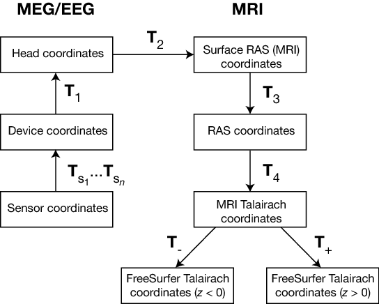
MEG/EEG and MRI coordinate systems

The coordinate transforms present in the fif files in MNE and the FreeSurfer files as well as those set to fixed values are indicated with \(T_x\), where \(x\) identifies the transformation.

The coordinate systems related to MEG/EEG data are:

Head coordinates

This is a coordinate system defined with help of the fiducial landmarks (nasion and the two auricular points). In fif files, EEG electrode locations are given in this coordinate system. In addition, the head digitization data acquired in the beginning of an MEG, MEG/EEG, or EEG acquisition are expressed in head coordinates. For details, see MEG/EEG and MRI coordinate systems.

Device coordinates

This is a coordinate system tied to the MEG device. The relationship of the Device and Head coordinates is determined during an MEG measurement by feeding current to three to five head-position indicator (HPI) coils and by determining their locations with respect to the MEG sensor array from the magnetic fields they generate.

Sensor coordinates

Each MEG sensor has a local coordinate system defining the orientation and location of the sensor. With help of this coordinate system, the numerical integration data needed for the computation of the magnetic field can be expressed conveniently as discussed in Coil geometry information. The channel information data in the fif files contain the information to specify the coordinate transformation between the coordinates of each sensor and the MEG device coordinates.

The coordinate systems related to MRI data are:

Surface RAS coordinates

The FreeSurfer surface data are expressed in this coordinate system. The origin of this coordinate system is at the center of the conformed FreeSurfer MRI volumes (usually 256 x 256 x 256 isotropic 1-mm3 voxels) and the axes are oriented along the axes of this volume. The BEM surface and the locations of the sources in the source space are usually expressed in this coordinate system in the fif files. In this manual, the Surface RAS coordinates are usually referred to as MRI coordinates unless there is need to specifically discuss the different MRI-related coordinate systems.

RAS coordinates

This coordinate system has axes identical to the Surface RAS coordinates but the location of the origin is different and defined by the original MRI data, i.e. , the origin is in a scanner-dependent location. There is hardly any need to refer to this coordinate system explicitly in the analysis with the MNE software. However, since the Talairach coordinates, discussed below, are defined with respect to RAS coordinates rather than the Surface RAS coordinates, the RAS coordinate system is implicitly involved in the transformation between Surface RAS coordinates and the two Talairach coordinate systems.

MNI Talairach coordinates

The definition of this coordinate system is discussed, e.g., in https://imaging.mrc-cbu.cam.ac.uk/imaging/MniTalairach. This transformation is determined during the FreeSurfer reconstruction process. These coordinates are in MNI305 space.

FreeSurfer Talairach coordinates

The problem with the MNI Talairach coordinates is that the linear MNI Talairach transform does not match the brains completely to the Talairach brain. This is probably because the Talairach atlas brain is a rather odd shape, and as a result, it is difficult to match a standard brain to the atlas brain using an affine transform. As a result, the MNI brains are slightly larger (in particular higher, deeper and longer) than the Talairach brain. The differences are larger as you get further from the middle of the brain, towards the outside. The FreeSurfer Talairach coordinates mitigate this problem by additing a an additional transformation, defined separately for negatice and positive MNI Talairach \(z\) coordinates. These two transformations, denoted by \(T_-\) and \(T_+\) in MEG/EEG and MRI coordinate systems, are fixed as discussed in https://imaging.mrc-cbu.cam.ac.uk/imaging/MniTalairach (Approach 2).

The different coordinate systems are related by coordinate transformations depicted in MEG/EEG and MRI coordinate systems. The arrows and coordinate transformation symbols (\(T_x\)) indicate the transformations actually present in the FreeSurfer files. Generally,

\[\begin{split}\begin{bmatrix} x_2 \\ y_2 \\ z_2 \\ 1 \end{bmatrix} = T_{12} \begin{bmatrix} x_1 \\ y_1 \\ z_1 \\ 1 \end{bmatrix} = \begin{bmatrix} R_{11} & R_{12} & R_{13} & x_0 \\ R_{21} & R_{22} & R_{23} & y_0 \\ R_{31} & R_{32} & R_{33} & z_0 \\ 0 & 0 & 0 & 1 \end{bmatrix} \begin{bmatrix} x_1 \\ y_1 \\ z_1 \\ 1 \end{bmatrix}\ ,\end{split}\]

where \(x_k\), \(y_k\),and \(z_k\) are the location coordinates in two coordinate systems, \(T_{12}\) is the coordinate transformation from coordinate system “1” to “2”, \(x_0\), \(y_0\), and \(z_0\) is the location of the origin of coordinate system “1” in coordinate system “2”, and \(R_{jk}\) are the elements of the rotation matrix relating the two coordinate systems. The coordinate transformations are present in different files produced by FreeSurfer and MNE. The fixed transformations \(T_-\) and \(T_+\) are:

\[\begin{split}T_{-} = \begin{bmatrix} 0.99 & 0 & 0 & 0 \\ 0 & 0.9688 & 0.042 & 0 \\ 0 & -0.0485 & 0.839 & 0 \\ 0 & 0 & 0 & 1 \end{bmatrix}\end{split}\]

and

\[\begin{split}T_{+} = \begin{bmatrix} 0.99 & 0 & 0 & 0 \\ 0 & 0.9688 & 0.046 & 0 \\ 0 & -0.0485 & 0.9189 & 0 \\ 0 & 0 & 0 & 1 \end{bmatrix}\end{split}\]

Note

This section does not discuss the transformation between the MRI voxel indices and the different MRI coordinates. However, it is important to note that in FreeSurfer, MNE, as well as in Neuromag software an integer voxel coordinate corresponds to the location of the center of a voxel. Detailed information on the FreeSurfer MRI systems can be found at https://surfer.nmr.mgh.harvard.edu/fswiki/CoordinateSystems. The symbols \(T_x\) are defined in MEG/EEG and MRI coordinate systems.

Coordinate transformations in FreeSurfer and MNE software packages.

Transformation	FreeSurfer	MNE
\(T_1\)	Not present	Measurement data files Forward solution files (*fwd.fif) Inverse operator files (*inv.fif)
\(T_{s_1}\dots T_{s_n}\)	Not present	Channel information in files containing \(T_1\).
\(T_2\)	Not present	MRI description filesSeparate Separate -trans.fif files from mne coreg Forward solution files Inverse operator files
\(T_3\)	mri/*mgz files	nibabel.freesurfer.mghformat.MGHImage
\(T_4\)	mri/transforms/talairach.xfm	Internal reading
\(T_-\)	Hardcoded in software	Hardcoded in software.
\(T_+\)	Hardcoded in software	Hardcoded in software.

The head and device coordinate systems

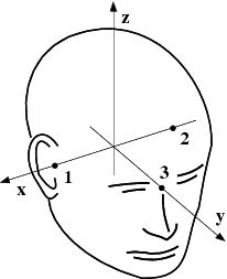
The head coordinate system

The MEG/EEG head coordinate system employed in the MNE software is a right-handed Cartesian coordinate system. The direction of \(x\) axis is from left to right, that of \(y\) axis to the front, and the \(z\) axis thus points up.

The \(x\) axis of the head coordinate system passes through the two periauricular or preauricular points digitized before acquiring the data with positive direction to the right. The \(y\) axis passes through the nasion and is normal to the \(x\) axis. The \(z\) axis points up according to the right-hand rule and is normal to the \(xy\) plane.

The origin of the MEG device coordinate system is device dependent. Its origin is located approximately at the center of a sphere which fits the occipital section of the MEG helmet best with \(x\) axis axis going from left to right and \(y\) axis pointing front. The \(z\) axis is, again, normal to the \(xy\) plane with positive direction up.

Note

The above definition is identical to that of the Neuromag MEG/EEG (head) coordinate system. However, in 4-D Neuroimaging and CTF MEG systems the head coordinate frame definition is different. The origin of the coordinate system is at the midpoint of the left and right auricular points. The \(x\) axis passes through the nasion and the origin with positive direction to the front. The \(y\) axis is perpendicular to the \(x\) axis on the and lies in the plane defined by the three fiducial landmarks, positive direction from right to left. The \(z\) axis is normal to the plane of the landmarks, pointing up. Note that in this convention the auricular points are not necessarily located on \(y\) coordinate axis. The file conversion utilities take care of these idiosyncrasies and convert all coordinate information to the MNE software head coordinate frame.

Creating a surface-based source space

The fif format source space files containing the dipole locations and orientations are created with mne.setup_source_space().

Creating a volumetric or discrete source space

In addition to source spaces confined to a surface, the MNE software provides some support for three-dimensional source spaces bounded by a surface as well as source spaces comprised of discrete, arbitrarily located source points. The mne.setup_volume_source_space() utility assists in generating such source spaces.

Creating the BEM meshes

See The Boundary Element Model (BEM).

Topology checks

The following topology checks are performed during the creation of BEM models:

• The completeness of each surface is confirmed by calculating the total solid angle subtended by all triangles from a point inside the triangulation. The result should be very close to \(4 \pi\). If the result is \(-4 \pi\) instead, it is conceivable that the ordering of the triangle vertices is incorrect and the --swap option should be specified.

• The correct ordering of the surfaces is verified by checking that the surfaces are inside each other as expected. This is accomplished by checking that the sum solid angles subtended by triangles of a surface \(S_k\) at all vertices of another surface \(S_p\) which is supposed to be inside it equals \(4 \pi\). Naturally, this check is applied only if the model has more than one surface. Since the surface relations are transitive, it is enough to check that the outer skull surface is inside the skin surface and that the inner skull surface is inside the outer skull one.

• The extent of each of the triangulated volumes is checked. If the extent is smaller than 50mm, an error is reported. This may indicate that the vertex coordinates have been specified in meters instead of millimeters.

Computing the BEM geometry data

The utility mne.make_bem_solution() computes the geometry information for BEM.

Coil geometry information

This Section explains the presentation of MEG detection coil geometry information the approximations used for different detection coils in MNE software. Two pieces of information are needed to characterize the detectors:

• The location and orientation a local coordinate system for each detector.

• A unique identifier, which has an one-to-one correspondence to the geometrical description of the coil.

Note

MNE ships with several coil geometry configurations. They can be found in mne/data. See Plotting sensor layouts of MEG systems for a comparison between different coil geometries, and Implemented coil geometries for detailed information regarding the files describing Neuromag coil geometries.

The sensor coordinate system

The sensor coordinate system is completely characterized by the location of its origin and the direction cosines of three orthogonal unit vectors pointing to the directions of the x, y, and z axis. In fact, the unit vectors contain redundant information because the orientation can be uniquely defined with three angles. The measurement fif files list these data in MEG device coordinates. Transformation to the MEG head coordinate frame can be easily accomplished by applying the device-to-head coordinate transformation matrix available in the data files provided that the head-position indicator was used. Optionally, the MNE software forward calculation applies another coordinate transformation to the head-coordinate data to bring the coil locations and orientations to the MRI coordinate system.

If \(r_0\) is a row vector for the origin of the local sensor coordinate system and \(e_x\), \(e_y\), and \(e_z\) are the row vectors for the three orthogonal unit vectors, all given in device coordinates, a location of a point \(r_C\) in sensor coordinates is transformed to device coordinates (\(r_D\)) by

\[[r_D 1] = [r_C 1] T_{CD}\ ,\]

where

\[\begin{split}T = \begin{bmatrix} e_x & 0 \\ e_y & 0 \\ e_z & 0 \\ r_{0D} & 1 \end{bmatrix}\ .\end{split}\]

Calculation of the magnetic field

The forward calculation in the MNE software computes the signals detected by each MEG sensor for three orthogonal dipoles at each source space location. This requires specification of the conductor model, the location and orientation of the dipoles, and the location and orientation of each MEG sensor as well as its coil geometry.

The output of each SQUID sensor is a weighted sum of the magnetic fluxes threading the loops comprising the detection coil. Since the flux threading a coil loop is an integral of the magnetic field component normal to the coil plane, the output of the k ^th MEG channel, \(b_k\) can be approximated by:

\[b_k = \sum_{p = 1}^{N_k} {w_{kp} B(r_{kp}) \cdot n_{kp}}\]

where \(r_{kp}\) are a set of \(N_k\) integration points covering the pickup coil loops of the sensor, \(B(r_{kp})\) is the magnetic field due to the current sources calculated at \(r_{kp}\), \(n_{kp}\) are the coil normal directions at these points, and \(w_{kp}\) are the weights associated to the integration points. This formula essentially presents numerical integration of the magnetic field over the pickup loops of sensor \(k\).

There are three accuracy levels for the numerical integration expressed above. The simple accuracy means the simplest description of the coil. This accuracy is not used in the MNE forward calculations. The normal or recommended accuracy typically uses two integration points for planar gradiometers, one in each half of the pickup coil and four evenly distributed integration points for magnetometers. This is the default accuracy used by MNE. If the --accurate option is specified, the forward calculation typically employs a total of eight integration points for planar gradiometers and sixteen for magnetometers. Detailed information about the integration points is given in the next section.

Implemented coil geometries

This section describes the coil geometries currently implemented in MNE. The coil types fall in two general categories:

• Axial gradiometers and planar gradiometers and

• Planar magnetometers.

For axial sensors, the z axis of the local coordinate system is parallel to the field component detected, i.e., normal to the coil plane.For circular coils, the orientation of the x and y axes on the plane normal to the z axis is irrelevant. In the square coils employed in the Vectorview (TM) system the x axis is chosen to be parallel to one of the sides of the magnetometer coil. For planar sensors, the z axis is likewise normal to the coil plane and the x axis passes through the centerpoints of the two coil loops so that the detector gives a positive signal when the normal field component increases along the x axis.

Normal coil descriptions. lists the parameters of the normal coil geometry descriptions Accurate coil descriptions lists the accurate descriptions. For simple accuracy, please consult the coil definition file, see The coil definition file. The columns of the tables contain the following data:

• The number identifying the coil id. This number is used in the coil descriptions found in the FIF files.

• Description of the coil.

• Number of integration points used

• The locations of the integration points in sensor coordinates.

• Weights assigned to the field values at the integration points. Some formulas are listed instead of the numerical values to demonstrate the principle of the calculation. For example, in the normal coil descriptions of the planar gradiometers the weights are inverses of the baseline of the gradiometer to show that the output is in T/m.

Note

The coil geometry information is stored in the file mne/data/coil_def.dat, which is automatically created by the MNE-C utility mne_list_coil_def.

Normal coil descriptions.

Id	Description	n	r/mm	w
2	Neuromag-122 planar gradiometer	2	(+/-8.1, 0, 0) mm	+/-1 ⁄ 16.2mm
2000	A point magnetometer	1	(0, 0, 0)mm	1
3012	Vectorview type 1 planar gradiometer	2	(+/-8.4, 0, 0.3) mm	+/-1 ⁄ 16.8mm
3013	Vectorview type 2 planar gradiometer	2	(+/-8.4, 0, 0.3) mm	+/-1 ⁄ 16.8mm
3022	Vectorview type 1 magnetometer	4	(+/-6.45, +/-6.45, 0.3)mm	1/4
3023	Vectorview type 2 magnetometer	4	(+/-6.45, +/-6.45, 0.3)mm	1/4
3024	Vectorview type 3 magnetometer	4	(+/-5.25, +/-5.25, 0.3)mm	1/4
2000	An ideal point magnetometer	1	(0.0, 0.0, 0.0)mm	1
4001	Magnes WH magnetometer	4	(+/-5.75, +/-5.75, 0.0)mm	1/4
4002	Magnes WH 3600 axial gradiometer	8	(+/-4.5, +/-4.5, 0.0)mm (+/-4.5, +/-4.5, 50.0)mm	1/4 -1/4
4003	Magnes reference magnetometer	4	(+/-7.5, +/-7.5, 0.0)mm	1/4
4004	Magnes reference gradiometer measuring diagonal gradients	8	(+/-20, +/-20, 0.0)mm (+/-20, +/-20, 135)mm	1/4 -1/4
4005	Magnes reference gradiometer measuring off-diagonal gradients	8	(87.5, +/-20, 0.0)mm (47.5, +/-20, 0.0)mm (-87.5, +/-20, 0.0)mm (-47.5, +/-20, 0.0)mm	1/4 -1/4 1/4 -1/4
5001	CTF 275 axial gradiometer	8	(+/-4.5, +/-4.5, 0.0)mm (+/-4.5, +/-4.5, 50.0)mm	1/4 -1/4
5002	CTF reference magnetometer	4	(+/-4, +/-4, 0.0)mm	1/4
5003	CTF reference gradiometer measuring diagonal gradients	8	(+/-8.6, +/-8.6, 0.0)mm (+/-8.6, +/-8.6, 78.6)mm	1/4 -1/4

Note

If a plus-minus sign occurs in several coordinates, all possible combinations have to be included.

Accurate coil descriptions

Id	Description	n	r/mm	w
2	Neuromag-122 planar gradiometer	8	+/-(8.1, 0, 0) mm	+/-1 ⁄ 16.2mm
2000	A point magnetometer	1	(0, 0, 0) mm	1
3012	Vectorview type 1 planar gradiometer	2	(+/-8.4, 0, 0.3) mm	+/-1 ⁄ 16.8mm
3013	Vectorview type 2 planar gradiometer	2	(+/-8.4, 0, 0.3) mm	+/-1 ⁄ 16.8mm
3022	Vectorview type 1 magnetometer	4	(+/-6.45, +/-6.45, 0.3)mm	1/4
3023	Vectorview type 2 magnetometer	4	(+/-6.45, +/-6.45, 0.3)mm	1/4
3024	Vectorview type 3 magnetometer	4	(+/-5.25, +/-5.25, 0.3)mm	1/4
4001	Magnes WH magnetometer	4	(+/-5.75, +/-5.75, 0.0)mm	1/4
4002	Magnes WH 3600 axial gradiometer	4	(+/-4.5, +/-4.5, 0.0)mm (+/-4.5, +/-4.5, 0.0)mm	1/4 -1/4
4004	Magnes reference gradiometer measuring diagonal gradients	8	(+/-20, +/-20, 0.0)mm (+/-20, +/-20, 135)mm	1/4 -1/4
4005	Magnes reference gradiometer measuring off-diagonal gradients	8	(87.5, +/-20, 0.0)mm (47.5, +/-20, 0.0)mm (-87.5, +/-20, 0.0)mm (-47.5, +/-20, 0.0)mm	1/4 -1/4 1/4 -1/4
5001	CTF 275 axial gradiometer	8	(+/-4.5, +/-4.5, 0.0)mm (+/-4.5, +/-4.5, 50.0)mm	1/4 -1/4
5002	CTF reference magnetometer	4	(+/-4, +/-4, 0.0)mm	1/4
5003	CTF 275 reference gradiometer measuring diagonal gradients	8	(+/-8.6, +/-8.6, 0.0)mm (+/-8.6, +/-8.6, 78.6)mm	1/4 -1/4
5004	CTF 275 reference gradiometer measuring off-diagonal gradients	8	(47.8, +/-8.5, 0.0)mm (30.8, +/-8.5, 0.0)mm (-47.8, +/-8.5, 0.0)mm (-30.8, +/-8.5, 0.0)mm	1/4 -1/4 1/4 -1/4
6001	MIT KIT system axial gradiometer	8	(+/-3.875, +/-3.875, 0.0)mm (+/-3.875, +/-3.875, 0.0)mm	1/4 -1/4

The coil definition file

The coil geometry information is stored in the text file $MNE_ROOT/share/mne/coil_def.dat. In this file, any lines starting with the pound sign (#) are comments. A coil definition starts with a description line containing the following fields:

• <class>: A number indicating class of this coil.

• <id>: Coil ID value. This value is listed in the first column of Tables Normal coil descriptions. and Accurate coil descriptions.

• <accuracy>: The coil representation accuracy. Possible values and their meanings are listed in Coil representation accuracies..

• <np>: Number of integration points in this representation.

• <size/m>: The size of the coil. For circular coils this is the diameter of the coil and for square ones the side length of the square. This information is mainly included to facilitate drawing of the coil geometry. It should not be employed to infer a coil approximation for the forward calculations.

• <baseline/m>: The baseline of a this kind of a coil. This will be zero for magnetometer coils. This information is mainly included to facilitate drawing of the coil geometry. It should not be employed to infer a coil approximation for the forward calculations.

• <description>: Short description of this kind of a coil. If the description contains several words, it is enclosed in quotes.

Coil representation accuracies.

Value	Meaning
1	The simplest representation available
2	The standard or normal representation (see Normal coil descriptions.)
3	The most accurate representation available (see Accurate coil descriptions)

Each coil description line is followed by one or more integration point lines, consisting of seven numbers:

• <weight>: Gives the weight for this integration point (last column in Tables Normal coil descriptions. and Accurate coil descriptions).

• <x/m> <y/m> <z/m>: Indicates the location of the integration point (fourth column in Tables Normal coil descriptions. and Accurate coil descriptions).

• <nx> <ny> <nz>: Components of a unit vector indicating the field component to be selected. Note that listing a separate unit vector for each integration points allows the implementation of curved coils and coils with the gradiometer loops tilted with respect to each other.

Computing the forward solution

Purpose

Examples on how to compute the forward solution in MNE-Python using mne.make_forward_solution() can be found Compute forward solution and Computing the forward solution.

Implementation of software gradient compensation

Accounting for noise cancellation in MNE-Python is accomplished in mne.io.Raw.apply_gradient_compensation(). See Brainstorm CTF phantom dataset tutorial for an example.

CTF and 4D Neuroimaging data may have been subjected to noise cancellation employing the data from the reference sensor array. Even though these sensor are rather far away from the brain sources, mne.make_forward_solution() takes them into account in the computations. If the data file has software gradient compensation activated, it computes the field of at the reference sensors in addition to the main MEG sensor array and computes a compensated forward solution.

The EEG sphere model definition file

In MNE-Python, different sphere models can be specified through mne.make_sphere_model(). The default model has the following structure:

Structure of the default EEG model

Layer	Relative outer radius	\(\sigma\) (S/m)
Head	1.0	0.33
Skull	0.97	0.04
CSF	0.92	1.0
Brain	0.90	0.33

Although it is not BEM model per se the sphere structure describes the head geometry so it can be passed as bem parameter in MNE-Python functions such as mne.fit_dipole(), mne.viz.plot_alignment() or mne.make_forward_solution().

EEG forward solution in the sphere model

Sphere-model examples in MNE-Python

For examples of using the sphere model when computing the forward model (using mne.make_forward_solution()), see Brainstorm CTF phantom dataset tutorial, Brainstorm Elekta phantom dataset tutorial, and Alignment without MRI.

When the sphere model is employed, the computation of the EEG solution can be substantially accelerated by using approximation methods described by Mosher 2, Zhang 3, and Berg 4. mne.make_forward_solution() approximates the solution with three dipoles in a homogeneous sphere whose locations and amplitudes are determined by minimizing the cost function:

\[S(r_1,\dotsc,r_m\ ,\ \mu_1,\dotsc,\mu_m) = \int_{scalp} {(V_{true} - V_{approx})}\,dS\]

where \(r_1,\dotsc,r_m\) and \(\mu_1,\dotsc,\mu_m\) are the locations and amplitudes of the approximating dipoles and \(V_{true}\) and \(V_{approx}\) are the potential distributions given by the true and approximative formulas, respectively. It can be shown that this integral can be expressed in closed form using an expansion of the potentials in spherical harmonics. The formula is evaluated for the most superficial dipoles, i.e., those lying just inside the inner skull surface.

Averaging forward solutions

One possibility to make a grand average over several runs of a experiment is to average the data across runs and average the forward solutions accordingly. For this purpose, mne.average_forward_solutions() computes a weighted average of several forward solutions. The function averages both MEG and EEG forward solutions. Usually the EEG forward solution is identical across runs because the electrode locations do not change.

The minimum-norm current estimates

This section describes the mathematical details of the calculation of minimum-norm estimates. In Bayesian sense, the ensuing current distribution is the maximum a posteriori (MAP) estimate under the following assumptions:

• The viable locations of the currents are constrained to the cortex. Optionally, the current orientations can be fixed to be normal to the cortical mantle.

• The amplitudes of the currents have a Gaussian prior distribution with a known source covariance matrix.

• The measured data contain additive noise with a Gaussian distribution with a known covariance matrix. The noise is not correlated over time.

Computing the inverse operator is accomplished using mne.minimum_norm.make_inverse_operator() and mne.minimum_norm.apply_inverse(). The use of these functions is presented in the tutorial Source localization with MNE/dSPM/sLORETA/eLORETA.

The linear inverse operator

The measured data in the source estimation procedure consists of MEG and EEG data, recorded on a total of N channels. The task is to estimate a total of \(Q\) strengths of sources located on the cortical mantle. If the number of source locations is \(P\), \(Q = P\) for fixed-orientation sources and \(Q = 3P\) if the source orientations are unconstrained. The regularized linear inverse operator following from regularized maximal likelihood of the above probabilistic model is given by the \(Q \times N\) matrix

\[M = R' G^\top (G R' G^\top + C)^{-1}\ ,\]

where \(G\) is the gain matrix relating the source strengths to the measured MEG/EEG data, \(C\) is the data noise-covariance matrix and \(R'\) is the source covariance matrix. The dimensions of these matrices are \(N \times Q\), \(N \times N\), and \(Q \times Q\), respectively. The \(Q \times 1\) source-strength vector is obtained by multiplying the \(Q \times 1\) data vector by \(Q\).

The expected value of the current amplitudes at time t is then given by \(\hat{j}(t) = Mx(t)\), where \(x(t)\) is a vector containing the measured MEG and EEG data values at time t.

For computational convenience, the linear inverse operator is not computed explicitly. See Computation of the solution for mathematical details, and Calculating the inverse operator for a detailed example.

Regularization

The a priori variance of the currents is, in practice, unknown. We can express this by writing \(R' = R/ \lambda^2 = R \lambda^{-2}\), which yields the inverse operator

(13)\[\begin{split} M &= R' G^\top (G R' G^\top + C)^{-1} \\ &= R \lambda^{-2} G^\top (G R \lambda^{-2} G^\top + C)^{-1} \\ &= R \lambda^{-2} G^\top \lambda^2 (G R G^\top + \lambda^2 C)^{-1} \\ &= R G^\top (G R G^\top + \lambda^2 C)^{-1}\ ,\end{split}\]

where the unknown current amplitude is now interpreted in terms of the regularization parameter \(\lambda^2\). Larger \(\lambda^2\) values correspond to spatially smoother and weaker current amplitudes, whereas smaller \(\lambda^2\) values lead to the opposite.

We can arrive at the regularized linear inverse operator also by minimizing a cost function \(S\) with respect to the estimated current \(\hat{j}\) (given the measurement vector \(x\) at any given time \(t\)) as

\[\begin{split}\min_\hat{j} \Bigl\{ S \Bigr\} &= \min_\hat{j} \Bigl\{ \tilde{e}^\top \tilde{e} + \lambda^2 \hat{j}^\top R^{-1} \hat{j} \Bigr\} \\ &= \min_\hat{j} \Bigl\{ (x - G\hat{j})^\top C^{-1} (x - G\hat{j}) + \lambda^2 \hat{j}^\top R^{-1} \hat{j} \Bigr\} \,\end{split}\]

where the first term consists of the difference between the whitened measured data (see Whitening and scaling) and those predicted by the model while the second term is a weighted-norm of the current estimate. It is seen that, with increasing \(\lambda^2\), the source term receive more weight and larger discrepancy between the measured and predicted data is tolerable.

Whitening and scaling

The MNE software employs data whitening so that a ‘whitened’ inverse operator assumes the form

(14)\[\tilde{M} = M C^{^1/_2} = R \tilde{G}^\top (\tilde{G} R \tilde{G}^\top + \lambda^2 I)^{-1}\ ,\]

where

(15)\[\tilde{G} = C^{-^1/_2}G\]

is the spatially whitened gain matrix. We arrive at the whitened inverse operator equation (14) by making the substitution for \(G\) from (15) in (13) as

\[\begin{split}\tilde{M} = M C^{^1/_2} &= R G^\top (G R G^\top + \lambda^2 C)^{-1} C^{^1/_2} \\ &= R \tilde{G}^\top C^{^1/_2} (C^{^1/_2} \tilde{G} R \tilde{G}^\top C^{^1/_2} + \lambda^2 C)^{-1} C^{^1/_2} \\ &= R \tilde{G}^\top C^{^1/_2} (C^{^1/_2} (\tilde{G} R \tilde{G}^\top + \lambda^2 I) C^{^1/_2})^{-1} C^{^1/_2} \\ &= R \tilde{G}^\top C^{^1/_2} C^{-^1/_2} (\tilde{G} R \tilde{G}^\top + \lambda^2 I)^{-1} C^{-^1/_2} C^{^1/_2} \\ &= R \tilde{G}^\top (\tilde{G} R \tilde{G}^\top + \lambda^2 I)^{-1}\ .\end{split}\]

The expected current values are

(16)\[\begin{split} \hat{j}(t) &= Mx(t) \\ &= M C^{^1/_2} C^{-^1/_2} x(t) \\ &= \tilde{M} \tilde{x}(t)\end{split}\]

knowing (14) and taking

(17)\[ \tilde{x}(t) = C^{-^1/_2}x(t)\]

as the whitened measurement vector at time t. The spatial whitening operator \(C^{-^1/_2}\) is obtained with the help of the eigenvalue decomposition \(C = U_C \Lambda_C^2 U_C^\top\) as \(C^{-^1/_2} = \Lambda_C^{-1} U_C^\top\). In the MNE software the noise-covariance matrix is stored as the one applying to raw data. To reflect the decrease of noise due to averaging, this matrix, \(C_0\), is scaled by the number of averages, \(L\), i.e., \(C = C_0 / L\).

As shown above, regularization of the inverse solution is equivalent to a change in the variance of the current amplitudes in the Bayesian a priori distribution.

A convenient choice for the source-covariance matrix \(R\) is such that \(\text{trace}(\tilde{G} R \tilde{G}^\top) / \text{trace}(I) = 1\). With this choice we can approximate \(\lambda^2 \sim 1/SNR\), where SNR is the (power) signal-to-noise ratio of the whitened data.

Note

The definition of the signal to noise-ratio/ \(\lambda^2\) relationship given above works nicely for the whitened forward solution. In the un-whitened case scaling with the trace ratio \(\text{trace}(GRG^\top) / \text{trace}(C)\) does not make sense, since the diagonal elements summed have, in general, different units of measure. For example, the MEG data are expressed in T or T/m whereas the unit of EEG is Volts.

See Computing a covariance matrix for example of noise covariance computation and whitening.

Regularization of the noise-covariance matrix

Since finite amount of data is usually available to compute an estimate of the noise-covariance matrix \(C\), the smallest eigenvalues of its estimate are usually inaccurate and smaller than the true eigenvalues. Depending on the seriousness of this problem, the following quantities can be affected:

• The model data predicted by the current estimate,

• Estimates of signal-to-noise ratios, which lead to estimates of the required regularization, see Regularization,

• The estimated current values, and

• The noise-normalized estimates, see Noise normalization.

Fortunately, the latter two are least likely to be affected due to regularization of the estimates. However, in some cases especially the EEG part of the noise-covariance matrix estimate can be deficient, i.e., it may possess very small eigenvalues and thus regularization of the noise-covariance matrix is advisable.

Historically, the MNE software accomplishes the regularization by replacing a noise-covariance matrix estimate \(C\) with

\[C' = C + \sum_k {\varepsilon_k \bar{\sigma_k}^2 I^{(k)}}\ ,\]

where the index \(k\) goes across the different channel groups (MEG planar gradiometers, MEG axial gradiometers and magnetometers, and EEG), \(\varepsilon_k\) are the corresponding regularization factors, \(\bar{\sigma_k}\) are the average variances across the channel groups, and \(I^{(k)}\) are diagonal matrices containing ones at the positions corresponding to the channels contained in each channel group.

See How should I regularize the covariance matrix? for details on computing and regularizing the channel covariance matrix.

Computation of the solution

The most straightforward approach to calculate the MNE is to employ the expression of the original or whitened inverse operator directly. However, for computational convenience we prefer to take another route, which employs the singular-value decomposition (SVD) of the matrix

(18)\[\begin{split} A &= \tilde{G} R^{^1/_2} \\ &= U \Lambda V^\top\end{split}\]

where the superscript \(^1/_2\) indicates a square root of \(R\). For a diagonal matrix, one simply takes the square root of \(R\) while in the more general case one can use the Cholesky factorization \(R = R_C R_C^\top\) and thus \(R^{^1/_2} = R_C\).

Combining the SVD from (18) with the inverse equation (13) it is easy to show that

(19)\[\begin{split} \tilde{M} &= R \tilde{G}^\top (\tilde{G} R \tilde{G}^\top + \lambda^2 I)^{-1} \\ &= R^{^1/_2} A^\top (A A^\top + \lambda^2 I)^{-1} \\ &= R^{^1/_2} V \Lambda U^\top (U \Lambda V^\top V \Lambda U^\top + \lambda^2 I)^{-1} \\ &= R^{^1/_2} V \Lambda U^\top (U (\Lambda^2 + \lambda^2 I) U^\top)^{-1} \\ &= R^{^1/_2} V \Lambda U^\top U (\Lambda^2 + \lambda^2 I)^{-1} U^\top \\ &= R^{^1/_2} V \Lambda (\Lambda^2 + \lambda^2 I)^{-1} U^\top \\ &= R^{^1/_2} V \Gamma U^\top\end{split}\]

where the elements of the diagonal matrix \(\Gamma\) are simply

(20)\[ \gamma_k = \frac{\lambda_k}{\lambda_k^2 + \lambda^2}\ .\]

From our expected current equation (16) and our whitened measurement equation (17), if we take

(21)\[\begin{split} w(t) &= U^\top \tilde{x}(t) \\ &= U^\top C^{-^1/_2} x(t)\ ,\end{split}\]

we can see that the expression for the expected current is just

(22)\[\begin{split} \hat{j}(t) &= R^{^1/_2} V \Gamma w(t) \\ &= \sum_k {\bar{v_k} \gamma_k w_k(t)}\ ,\end{split}\]

where \(\bar{v_k} = R^{^1/_2} v_k\), with \(v_k\) being the \(k\) th column of \(V\). It is thus seen that the current estimate is a weighted sum of the “weighted” eigenleads \(v_k\).

It is easy to see that \(w(t) \propto \sqrt{L}\). To maintain the relation \((\tilde{G} R \tilde{G}^\top) / \text{trace}(I) = 1\) when \(L\) changes we must have \(R \propto 1/L\). With this approach, \(\lambda_k\) is independent of \(L\) and, for fixed \(\lambda\), we see directly that \(j(t)\) is independent of \(L\).

The minimum-norm estimate is computed using this procedure in mne.minimum_norm.make_inverse_operator(), and its usage is illustrated in Calculating the inverse operator.

Noise normalization

Noise normalization serves three purposes:

• It converts the expected current value into a dimensionless statistical test variable. Thus the resulting time and location dependent values are often referred to as dynamic statistical parameter maps (dSPM).

• It reduces the location bias of the estimates. In particular, the tendency of the MNE to prefer superficial currents is eliminated.

• The width of the point-spread function becomes less dependent on the source location on the cortical mantle. The point-spread is defined as the MNE resulting from the signals coming from a point current source (a current dipole) located at a certain point on the cortex.

In practice, noise normalization is implemented as a division by the square root of the estimated variance of each voxel. In computing these noise normalization factors, it’s convenient to reuse our “weighted eigenleads” definition from equation (16) in matrix form as

(23)\[ \bar{V} = R^{^1/_2} V\ .\]

dSPM

Noise-normalized linear estimates introduced by Dale et al. 5 require division of the expected current amplitude by its variance. In practice, this requires the computation of the diagonal elements of the following matrix, using SVD equation (14) and (23):

\[\begin{split}M C M^\top &= M C^{^1/_2} C^{^1/_2} M^\top \\ &= \tilde{M} \tilde{M}^\top \\ &= R^{^1/_2} V \Gamma U^\top U \Gamma V^\top R^{^1/_2} \\ &= \bar{V} \Gamma^2 \bar{V}^\top\ .\end{split}\]

Because we only care about the diagonal entries here, we can find the variances for each source as

\[\sigma_k^2 = \gamma_k^2\]

Under the conditions expressed at the end of Computation of the solution, it follows that the t-statistic values associated with fixed-orientation sources) are thus proportional to \(\sqrt{L}\) while the F-statistic employed with free-orientation sources is proportional to \(L\), correspondingly.

Note

The MNE software usually computes the square roots of the F-statistic to be displayed on the inflated cortical surfaces. These are also proportional to \(\sqrt{L}\).

sLORETA

sLORETA 6 estimates the current variances as the diagonal entries of the resolution matrix, which is the product of the inverse and forward operators. In other words, the diagonal entries of (using (19), (15), and (18))

\[\begin{split}M G &= M C^{^1/_2} C^{-^1/_2} G \\ &= \tilde{M} \tilde{G} \\ &= R^{^1/_2} V \Gamma U^\top \tilde{G} R^{^1/_2} R^{-^1/_2} \\ &= R^{^1/_2} V \Gamma U^\top U \Lambda V^\top R^{-^1/_2} \\ &= R^{^1/_2} V \Gamma U^\top U \Lambda V^\top R^{^1/_2} R^{-1} \\ &= \bar{V} \Gamma U^\top U \Lambda \bar{V}^\top R^{-1} \\ &= \bar{V} \Gamma \Lambda \bar{V}^\top R^{-1}\ .\end{split}\]

Because \(R\) is diagonal and we only care about the diagonal entries, we can find our variance estimates as

\[\begin{split}\sigma_k^2 &= \gamma_k \lambda_k R_{k,k}^{-1} \\ &= \left(\frac{\lambda_k}{(\lambda_k^2 + \lambda^2)}\right) \left(\frac{\lambda_k}{1}\right) \left(\frac{1}{\lambda^2}\right) \\ &= \frac{\lambda_k^2}{(\lambda_k^2 + \lambda^2) \lambda^2} \\ &= \left(\frac{\lambda_k^2}{(\lambda_k^2 + \lambda^2)^2}\right) \left(\frac{\lambda^2 + \lambda_k^2}{\lambda^2}\right) \\ &= \left(\frac{\lambda_k}{\lambda_k^2 + \lambda^2}\right)^2 \left(1 + \frac{\lambda_k^2}{\lambda^2}\right) \\ &= \gamma_k^2 \left(1 + \frac{\lambda_k^2}{\lambda^2}\right)\ .\end{split}\]

eLORETA

While dSPM and sLORETA solve for noise normalization weights \(\sigma^2_k\) that are applied to standard minimum-norm estimates \(\hat{j}(t)\), eLORETA 7 instead solves for a source covariance matrix \(R\) that achieves zero localization bias. For fixed-orientation solutions the resulting matrix \(R\) will be a diagonal matrix, and for free-orientation solutions it will be a block-diagonal matrix with \(3 \times 3\) blocks.

In 7 eq. 2.13 states that the following system of equations can be used to find the weights, \(\forall i \in {1, ..., P}\) (note that here we represent the equations from that paper using our notation):

\[r_i = \left[ G_i^\top \left( GRG^\top + \lambda^2C \right)^{-1} G_i \right] ^{-^1/_2}\]

And an iterative algorithm can be used to find the values for the weights \(r_i\) that satisfy these equations as:

1. Initialize identity weights.

2. Compute \(N= \left( GRG^\top + \lambda^2C \right)^{-1}\).

3. Holding \(N\) fixed, compute new weights \(r_i = \left[ G_i^\top N G_i \right]^{-^1/_2}\).

4. Using new weights, go to step (2) until convergence.

In particular, for step (2) we can use our substitution from (15) as:

\[\begin{split}N &= (G R G^\top + \lambda^2 C)^{-1} \\ &= (C^{^1/_2} \tilde{G} R \tilde{G}^\top C^{^1/_2} + \lambda^2 C)^{-1} \\ &= (C^{^1/_2} (\tilde{G} R \tilde{G}^\top + \lambda^2 I) C^{^1/_2})^{-1} \\ &= C^{-^1/_2} (\tilde{G} R \tilde{G}^\top + \lambda^2 I)^{-1} C^{-^1/_2} \\ &= C^{-^1/_2} (\tilde{G} R \tilde{G}^\top + \lambda^2 I)^{-1} C^{-^1/_2}\ .\end{split}\]

Then defining \(\tilde{N}\) as the whitened version of \(N\), i.e., the regularized pseudoinverse of \(\tilde{G}R\tilde{G}^\top\), we can compute \(N\) as:

\[\begin{split}N &= C^{-^1/_2} (U_{\tilde{G}R\tilde{G}^\top} \Lambda_{\tilde{G}R\tilde{G}^\top} V_{\tilde{G}R\tilde{G}^\top}^\top + \lambda^2 I)^{-1} C^{-^1/_2} \\ &= C^{-^1/_2} (U_{\tilde{G}R\tilde{G}^\top} (\Lambda_{\tilde{G}R\tilde{G}^\top} + \lambda^2 I) V_{\tilde{G}R\tilde{G}^\top}^\top)^{-1} C^{-^1/_2} \\ &= C^{-^1/_2} V_{\tilde{G}R\tilde{G}^\top} (\Lambda_{\tilde{G}R\tilde{G}^\top} + \lambda^2 I)^{-1} U_{\tilde{G}R\tilde{G}^\top}^\top C^{-^1/_2} \\ &= C^{-^1/_2} \tilde{N} C^{-^1/_2}\ .\end{split}\]

In step (3) we left and right multiply with subsets of \(G\), but making the substitution (15) we see that we equivalently compute:

\[\begin{split}r_i &= \left[ G_i^\top N G_i \right]^{-^1/_2} \\ &= \left[ (C^{^1/_2} \tilde{G}_i)^\top N C^{^1/_2} \tilde{G}_i \right]^{-^1/_2} \\ &= \left[ \tilde{G}_i^\top C^{^1/_2} N C^{^1/_2} \tilde{G}_i \right]^{-^1/_2} \\ &= \left[ \tilde{G}_i^\top C^{^1/_2} C^{-^1/_2} \tilde{N} C^{-^1/_2} C^{^1/_2} \tilde{G}_i \right]^{-^1/_2} \\ &= \left[ \tilde{G}_i^\top \tilde{N} \tilde{G}_i \right]^{-^1/_2}\ .\end{split}\]

For convenience, we thus never need to compute \(N\) itself but can instead compute the whitened version \(\tilde{N}\).

Predicted data

Under noiseless conditions the SNR is infinite and thus leads to \(\lambda^2 = 0\) and the minimum-norm estimate explains the measured data perfectly. Under realistic conditions, however, \(\lambda^2 > 0\) and there is a misfit between measured data and those predicted by the MNE. Comparison of the predicted data, here denoted by \(x(t)\), and measured one can give valuable insight on the correctness of the regularization applied.

In the SVD approach we easily find

\[\hat{x}(t) = G \hat{j}(t) = C^{^1/_2} U \Pi w(t)\ ,\]

where the diagonal matrix \(\Pi\) has elements \(\pi_k = \lambda_k \gamma_k\) The predicted data is thus expressed as the weighted sum of the ‘recolored eigenfields’ in \(C^{^1/_2} U\).

Cortical patch statistics

If the add_dists=True option was used in source space creation, the source space file will contain Cortical Patch Statistics (CPS) for each vertex of the cortical surface. The CPS provide information about the source space point closest to it as well as the distance from the vertex to this source space point. The vertices for which a given source space point is the nearest one define the cortical patch associated with with the source space point. Once these data are available, it is straightforward to compute the following cortical patch statistics for each source location \(d\):

• The average over the normals of at the vertices in a patch, \(\bar{n_d}\),

• The areas of the patches, \(A_d\), and

• The average deviation of the vertex normals in a patch from their average, \(\sigma_d\), given in degrees.

use_cps parameter in mne.convert_forward_solution(), and mne.minimum_norm.make_inverse_operator() controls whether to use cortical patch statistics (CPS) to define normal orientations or not (see Cortical surface reconstruction with FreeSurfer).

Orientation constraints

The principal sources of MEG and EEG signals are generally believed to be postsynaptic currents in the cortical pyramidal neurons. Since the net primary current associated with these microscopic events is oriented normal to the cortical mantle, it is reasonable to use the cortical normal orientation as a constraint in source estimation. In addition to allowing completely free source orientations, the MNE software implements three orientation constraints based of the surface normal data:

• Source orientation can be rigidly fixed to the surface normal direction by specifying fixed=True in mne.minimum_norm.make_inverse_operator(). If cortical patch statistics are available the average normal over each patch, \(\bar{n_d}\), are used to define the source orientation. Otherwise, the vertex normal at the source space location is employed.

• A location independent or fixed loose orientation constraint (fLOC) can be employed by specifying fixed=False and loose=1.0 when calling mne.minimum_norm.make_inverse_operator() (see Loose dipole orientations). In this approach, a source coordinate system based on the local surface orientation at the source location is employed. By default, the three columns of the gain matrix G, associated with a given source location, are the fields of unit dipoles pointing to the directions of the \(x\), \(y\), and \(z\) axis of the coordinate system employed in the forward calculation (usually the MEG head coordinate frame). For LOC the orientation is changed so that the first two source components lie in the plane normal to the surface normal at the source location and the third component is aligned with it. Thereafter, the variance of the source components tangential to the cortical surface are reduced by a factor defined by the --loose option.

• A variable loose orientation constraint (vLOC) can be employed by specifying fixed=False and loose parameters when calling mne.minimum_norm.make_inverse_operator() (see Limiting orientations, but not fixing them). This is similar to fLOC except that the value given with the loose parameter will be multiplied by \(\sigma_d\), defined above.

Depth weighting

The minimum-norm estimates have a bias towards superficial currents. This tendency can be alleviated by adjusting the source covariance matrix \(R\) to favor deeper source locations. In the depth weighting scheme employed in MNE analyze, the elements of \(R\) corresponding to the \(p\) th source location are be scaled by a factor

\[f_p = (g_{1p}^\top g_{1p} + g_{2p}^\top g_{2p} + g_{3p}^\top g_{3p})^{-\gamma}\ ,\]

where \(g_{1p}\), \(g_{2p}\), and \(g_{3p}\) are the three columns of \(G\) corresponding to source location \(p\) and \(\gamma\) is the order of the depth weighting, which is specified via the depth option in mne.minimum_norm.make_inverse_operator().

Effective number of averages

It is often the case that the epoch to be analyzed is a linear combination over conditions rather than one of the original averages computed. As stated above, the noise-covariance matrix computed is originally one corresponding to raw data. Therefore, it has to be scaled correctly to correspond to the actual or effective number of epochs in the condition to be analyzed. In general, we have

\[C = C_0 / L_{eff}\]

where \(L_{eff}\) is the effective number of averages. To calculate \(L_{eff}\) for an arbitrary linear combination of conditions

\[y(t) = \sum_{i = 1}^n {w_i x_i(t)}\]

we make use of the the fact that the noise-covariance matrix

\[C_y = \sum_{i = 1}^n {w_i^2 C_{x_i}} = C_0 \sum_{i = 1}^n {w_i^2 / L_i}\]

which leads to

\[1 / L_{eff} = \sum_{i = 1}^n {w_i^2 / L_i}\]

An important special case of the above is a weighted average, where

\[w_i = L_i / \sum_{i = 1}^n {L_i}\]

and, therefore

\[L_{eff} = \sum_{i = 1}^n {L_i}\]

Instead of a weighted average, one often computes a weighted sum, a simplest case being a difference or sum of two categories. For a difference \(w_1 = 1\) and \(w_2 = -1\) and thus

\[1 / L_{eff} = 1 / L_1 + 1 / L_2\]

or

\[L_{eff} = \frac{L_1 L_2}{L_1 + L_2}\]

Interestingly, the same holds for a sum, where \(w_1 = w_2 = 1\). Generalizing, for any combination of sums and differences, where \(w_i = 1\) or \(w_i = -1\), \(i = 1 \dotso n\), we have

\[1 / L_{eff} = \sum_{i = 1}^n {1/{L_i}}\]

Morphing and averaging source estimates

Why morphing?

Morphing examples in MNE-Python

Examples of morphing in MNE-Python include this tutorial on surface source estimation or these examples on surface and volumetric source estimation.

Modern neuroimaging techniques, such as source reconstruction or fMRI analyses, make use of advanced mathematical models and hardware to map brain activity patterns into a subject-specific anatomical brain space. This enables the study of spatio-temporal brain activity. The representation of spatio-temporal brain data is often mapped onto the anatomical brain structure to relate functional and anatomical maps. Thereby activity patterns are overlaid with anatomical locations that supposedly produced the activity. Anatomical MR images are often used as such or are transformed into an inflated surface representations to serve as “canvas” for the visualization.

In order to compute group-level statistics, data representations across subjects must be morphed to a common frame, such that anatomically and functional similar structures are represented at the same spatial location for all subjects equally. Since brains vary, morphing comes into play to tell us how the data produced by subject A would be represented on the brain of subject B (and vice-versa).

The morphing maps

The MNE software accomplishes morphing with help of morphing maps. The morphing is performed with help of the registered spherical surfaces (lh.sphere.reg and rh.sphere.reg ) which must be produced in FreeSurfer. A morphing map is a linear mapping from cortical surface values in subject A (\(x^{(A)}\)) to those in another subject B (\(x^{(B)}\))

\[x^{(B)} = M^{(AB)} x^{(A)}\ ,\]

where \(M^{(AB)}\) is a sparse matrix with at most three nonzero elements on each row. These elements are determined as follows. First, using the aligned spherical surfaces, for each vertex \(x_j^{(B)}\), find the triangle \(T_j^{(A)}\) on the spherical surface of subject A which contains the location \(x_j^{(B)}\). Next, find the numbers of the vertices of this triangle and set the corresponding elements on the j th row of \(M^{(AB)}\) so that \(x_j^{(B)}\) will be a linear interpolation between the triangle vertex values reflecting the location \(x_j^{(B)}\) within the triangle \(T_j^{(A)}\).

It follows from the above definition that in general

\[M^{(AB)} \neq (M^{(BA)})^{-1}\ ,\]

i.e.,

\[x_{(A)} \neq M^{(BA)} M^{(AB)} x^{(A)}\ ,\]

even if

\[x^{(A)} \approx M^{(BA)} M^{(AB)} x^{(A)}\ ,\]

i.e., the mapping is almost a bijection.

About smoothing

The current estimates are normally defined only in a decimated grid which is a sparse subset of the vertices in the triangular tessellation of the cortical surface. Therefore, any sparse set of values is distributed to neighboring vertices to make the visualized results easily understandable. This procedure has been traditionally called smoothing but a more appropriate name might be smudging or blurring in accordance with similar operations in image processing programs.

In MNE software terms, smoothing of the vertex data is an iterative procedure, which produces a blurred image \(x^{(N)}\) from the original sparse image \(x^{(0)}\) by applying in each iteration step a sparse blurring matrix:

\[x^{(p)} = S^{(p)} x^{(p - 1)}\ .\]

On each row \(j\) of the matrix \(S^{(p)}\) there are \(N_j^{(p - 1)}\) nonzero entries whose values equal \(1/N_j^{(p - 1)}\). Here \(N_j^{(p - 1)}\) is the number of immediate neighbors of vertex \(j\) which had non-zero values at iteration step \(p - 1\). Matrix \(S^{(p)}\) thus assigns the average of the non-zero neighbors as the new value for vertex \(j\). One important feature of this procedure is that it tends to preserve the amplitudes while blurring the surface image.

Once the indices non-zero vertices in \(x^{(0)}\) and the topology of the triangulation are fixed the matrices \(S^{(p)}\) are fixed and independent of the data. Therefore, it would be in principle possible to construct a composite blurring matrix

\[S^{(N)} = \prod_{p = 1}^N {S^{(p)}}\ .\]

However, it turns out to be computationally more effective to do blurring with an iteration. The above formula for \(S^{(N)}\) also shows that the smudging (smoothing) operation is linear.

References

1

François M. Perrin, Jacques Pernier, Olivier M. Bertrand, and Jean Franćois Echallier. Spherical splines for scalp potential and current density mapping. Electroencephalography and Clinical Neurophysiology, 72(2):184–187, 1989. doi:10.1016/0013-4694(89)90180-6.

2

John C. Mosher, Richard M. Leahy, and Paul S. Lewis. EEG and MEG: forward solutions for inverse methods. IEEE Transactions on Biomedical Engineering, 46(3):245–259, 1999. doi:10.1109/10.748978.

3

Zhi Zhang. A fast method to compute surface potentials generated by dipoles within multilayer anisotropic spheres. Physics in Medicine and Biology, 40(3):335–349, 1995. doi:10.1088/0031-9155/40/3/001.

4

Patrick Berg and Michael Scherg. A fast method for forward computation of multiple-shell spherical head models. Electroencephalography and Clinical Neurophysiology, 90(1):58–64, 1994. doi:10.1016/0013-4694(94)90113-9.

5

Anders M. Dale, Bruce Fischl, and Martin I. Sereno. Cortical surface-based analysis: I. segmentation and surface reconstruction. NeuroImage, 9(2):179–194, 1999. doi:10.1006/nimg.1998.0395.

6

Roberto D. Pascual-Marqui. Standardized low-resolution brain electromagnetic tomography (sLORETA): technical details. Methods and Findings in Experimental and Clinical Pharmacology, 24(D):5–12, 2002.

7(1,2)

Roberto D. Pascual-Marqui, Dietrich Lehmann, Martha Koukkou, Kieko Kochi, Peter Anderer, Bernd Saletu, Hideaki Tanaka, Koichi Hirata, E. Roy John, Leslie Prichep, Rolando Biscay-Lirio, and Toshihiko Kinoshita. Assessing interactions in the brain with exact low-resolution electromagnetic tomography. Philosophical Transactions of the Royal Society A: Mathematical, Physical and Engineering Sciences, 369(1952):3768–3784, October 2011. URL: https://royalsocietypublishing.org/doi/full/10.1098/rsta.2011.0081, doi:10.1098/rsta.2011.0081.