Note
Click here to download the full example code
Source localization with MNE/dSPM/sLORETA/eLORETA
The aim of this tutorial is to teach you how to compute and apply a linear minimum-norm inverse method on evoked/raw/epochs data.
import numpy as np
import matplotlib.pyplot as plt
import mne
from mne.datasets import sample
from mne.minimum_norm import make_inverse_operator, apply_inverse
Process MEG data
data_path = sample.data_path()
raw_fname = data_path + '/MEG/sample/sample_audvis_filt-0-40_raw.fif'
raw = mne.io.read_raw_fif(raw_fname) # already has an average reference
events = mne.find_events(raw, stim_channel='STI 014')
event_id = dict(aud_l=1) # event trigger and conditions
tmin = -0.2 # start of each epoch (200ms before the trigger)
tmax = 0.5 # end of each epoch (500ms after the trigger)
raw.info['bads'] = ['MEG 2443', 'EEG 053']
baseline = (None, 0) # means from the first instant to t = 0
reject = dict(grad=4000e-13, mag=4e-12, eog=150e-6)
epochs = mne.Epochs(raw, events, event_id, tmin, tmax, proj=True,
picks=('meg', 'eog'), baseline=baseline, reject=reject)
Out:
Opening raw data file /home/circleci/mne_data/MNE-sample-data/MEG/sample/sample_audvis_filt-0-40_raw.fif...
Read a total of 4 projection items:
PCA-v1 (1 x 10²) idle
PCA-v2 (1 x 10²) idle
PCA-v3 (1 x 10²) idle
Average EEG reference (1 x 60) idle
Range : 6450 ... 48149 = 42.956 ... 320.665 secs
Ready.
319 events found
Event IDs: [ 1 2 3 4 5 32]
Not setting metadata
Not setting metadata
72 matching events found
Setting baseline interval to [-0.19979521315838786, 0.0] sec
Applying baseline correction (mode: mean)
Created an SSP operator (subspace dimension = 3)
4 projection items activated
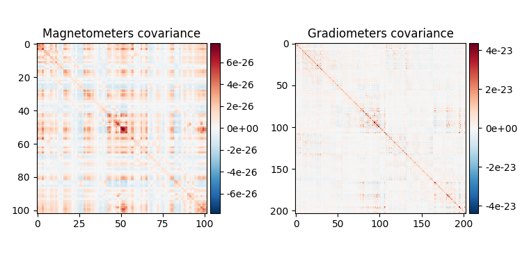
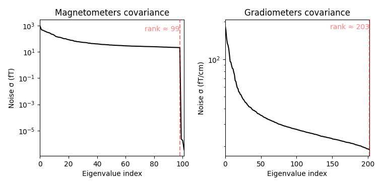
Compute regularized noise covariance
For more details see Computing a covariance matrix.
noise_cov = mne.compute_covariance(
epochs, tmax=0., method=['shrunk', 'empirical'], rank=None, verbose=True)
fig_cov, fig_spectra = mne.viz.plot_cov(noise_cov, raw.info)
Out:
Loading data for 72 events and 106 original time points ...
Rejecting epoch based on EOG : ['EOG 061']
Rejecting epoch based on EOG : ['EOG 061']
Rejecting epoch based on EOG : ['EOG 061']
Rejecting epoch based on EOG : ['EOG 061']
Rejecting epoch based on EOG : ['EOG 061']
Rejecting epoch based on MAG : ['MEG 1711']
Rejecting epoch based on EOG : ['EOG 061']
Rejecting epoch based on EOG : ['EOG 061']
Rejecting epoch based on EOG : ['EOG 061']
Rejecting epoch based on EOG : ['EOG 061']
Rejecting epoch based on EOG : ['EOG 061']
Rejecting epoch based on EOG : ['EOG 061']
Rejecting epoch based on EOG : ['EOG 061']
Rejecting epoch based on EOG : ['EOG 061']
Rejecting epoch based on EOG : ['EOG 061']
Rejecting epoch based on EOG : ['EOG 061']
Rejecting epoch based on EOG : ['EOG 061']
17 bad epochs dropped
Computing rank from data with rank=None
Using tolerance 2.8e-09 (2.2e-16 eps * 305 dim * 4.2e+04 max singular value)
Estimated rank (mag + grad): 302
MEG: rank 302 computed from 305 data channels with 3 projectors
Created an SSP operator (subspace dimension = 3)
Setting small MEG eigenvalues to zero (without PCA)
Reducing data rank from 305 -> 302
Estimating covariance using SHRUNK
Done.
Estimating covariance using EMPIRICAL
Done.
Using cross-validation to select the best estimator.
Number of samples used : 1705
log-likelihood on unseen data (descending order):
shrunk: -1466.595
empirical: -1574.608
selecting best estimator: shrunk
[done]
Computing rank from covariance with rank=None
Using tolerance 2.2e-14 (2.2e-16 eps * 102 dim * 0.97 max singular value)
Estimated rank (mag): 99
MAG: rank 99 computed from 102 data channels with 0 projectors
Computing rank from covariance with rank=None
Using tolerance 1.6e-13 (2.2e-16 eps * 203 dim * 3.4 max singular value)
Estimated rank (grad): 203
GRAD: rank 203 computed from 203 data channels with 0 projectors
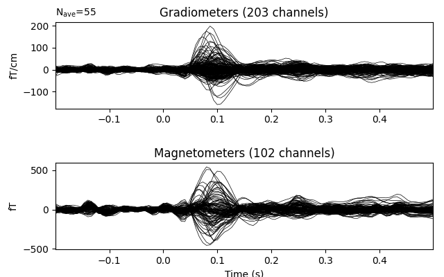
Compute the evoked response
Let’s just use the MEG channels for simplicity.
evoked = epochs.average().pick('meg')
evoked.plot(time_unit='s')
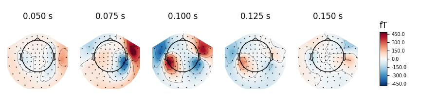
evoked.plot_topomap(times=np.linspace(0.05, 0.15, 5), ch_type='mag',
time_unit='s')
Out:
Removing projector <Projection | Average EEG reference, active : True, n_channels : 60>
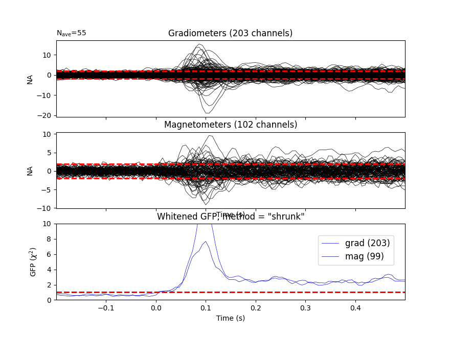
It’s also a good idea to look at whitened data:
evoked.plot_white(noise_cov, time_unit='s')
del epochs, raw # to save memory
Out:
Computing rank from covariance with rank=None
Using tolerance 1.6e-13 (2.2e-16 eps * 203 dim * 3.4 max singular value)
Estimated rank (grad): 203
GRAD: rank 203 computed from 203 data channels with 0 projectors
Computing rank from covariance with rank=None
Using tolerance 2.2e-14 (2.2e-16 eps * 102 dim * 0.97 max singular value)
Estimated rank (mag): 99
MAG: rank 99 computed from 102 data channels with 3 projectors
Created an SSP operator (subspace dimension = 3)
Computing rank from covariance with rank={'grad': 203, 'mag': 99, 'meg': 302}
Setting small MEG eigenvalues to zero (without PCA)
Created the whitener using a noise covariance matrix with rank 302 (3 small eigenvalues omitted)
Inverse modeling: MNE/dSPM on evoked and raw data
Here we first read the forward solution. You will likely need to compute one for your own data – see Head model and forward computation for information on how to do it.
fname_fwd = data_path + '/MEG/sample/sample_audvis-meg-oct-6-fwd.fif'
fwd = mne.read_forward_solution(fname_fwd)
Out:
Reading forward solution from /home/circleci/mne_data/MNE-sample-data/MEG/sample/sample_audvis-meg-oct-6-fwd.fif...
Reading a source space...
Computing patch statistics...
Patch information added...
Distance information added...
[done]
Reading a source space...
Computing patch statistics...
Patch information added...
Distance information added...
[done]
2 source spaces read
Desired named matrix (kind = 3523) not available
Read MEG forward solution (7498 sources, 306 channels, free orientations)
Source spaces transformed to the forward solution coordinate frame
Next, we make an MEG inverse operator.
inverse_operator = make_inverse_operator(
evoked.info, fwd, noise_cov, loose=0.2, depth=0.8)
del fwd
# You can write it to disk with::
#
# >>> from mne.minimum_norm import write_inverse_operator
# >>> write_inverse_operator('sample_audvis-meg-oct-6-inv.fif',
# inverse_operator)
Out:
Converting forward solution to surface orientation
Average patch normals will be employed in the rotation to the local surface coordinates....
Converting to surface-based source orientations...
[done]
info["bads"] and noise_cov["bads"] do not match, excluding bad channels from both
Computing inverse operator with 305 channels.
305 out of 306 channels remain after picking
Selected 305 channels
Creating the depth weighting matrix...
203 planar channels
limit = 7265/7498 = 10.037795
scale = 2.52065e-08 exp = 0.8
Applying loose dipole orientations to surface source spaces: 0.2
Whitening the forward solution.
Created an SSP operator (subspace dimension = 3)
Computing rank from covariance with rank=None
Using tolerance 2.9e-13 (2.2e-16 eps * 305 dim * 4.2 max singular value)
Estimated rank (mag + grad): 302
MEG: rank 302 computed from 305 data channels with 3 projectors
Setting small MEG eigenvalues to zero (without PCA)
Creating the source covariance matrix
Adjusting source covariance matrix.
Computing SVD of whitened and weighted lead field matrix.
largest singular value = 4.69422
scaling factor to adjust the trace = 8.8068e+18
Compute inverse solution
We can use this to compute the inverse solution and obtain source time courses:
Out:
Preparing the inverse operator for use...
Scaled noise and source covariance from nave = 1 to nave = 55
Created the regularized inverter
Created an SSP operator (subspace dimension = 3)
Created the whitener using a noise covariance matrix with rank 302 (3 small eigenvalues omitted)
Computing noise-normalization factors (dSPM)...
[done]
Applying inverse operator to "aud_l"...
Picked 305 channels from the data
Computing inverse...
Eigenleads need to be weighted ...
Computing residual...
Explained 66.0% variance
Combining the current components...
dSPM...
[done]
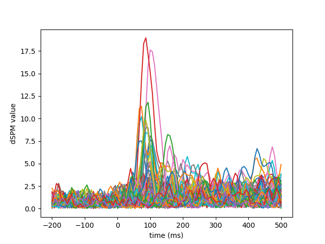
Visualization
We can look at different dipole activations:
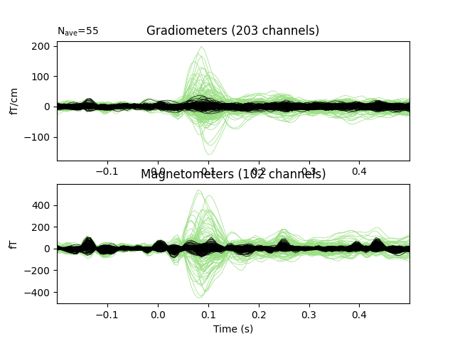
Examine the original data and the residual after fitting:
fig, axes = plt.subplots(2, 1)
evoked.plot(axes=axes)
for ax in axes:
ax.texts = []
for line in ax.lines:
line.set_color('#98df81')
residual.plot(axes=axes)
Here we use peak getter to move visualization to the time point of the peak and draw a marker at the maximum peak vertex.
vertno_max, time_max = stc.get_peak(hemi='rh')
subjects_dir = data_path + '/subjects'
surfer_kwargs = dict(
hemi='rh', subjects_dir=subjects_dir,
clim=dict(kind='value', lims=[8, 12, 15]), views='lateral',
initial_time=time_max, time_unit='s', size=(800, 800), smoothing_steps=10)
brain = stc.plot(**surfer_kwargs)
brain.add_foci(vertno_max, coords_as_verts=True, hemi='rh', color='blue',
scale_factor=0.6, alpha=0.5)
brain.add_text(0.1, 0.9, 'dSPM (plus location of maximal activation)', 'title',
font_size=14)
# The documentation website's movie is generated with:
# brain.save_movie(..., tmin=0.05, tmax=0.15, interpolation='linear',
# time_dilation=20, framerate=10, time_viewer=True)
There are many other ways to visualize and work with source data, see for example:
Total running time of the script: ( 0 minutes 47.985 seconds)
Estimated memory usage: 150 MB