Note
Click here to download the full example code
Non-parametric 1 sample cluster statistic on single trial power
This script shows how to estimate significant clusters in time-frequency power estimates. It uses a non-parametric statistical procedure based on permutations and cluster level statistics.
The procedure consists of:
extracting epochs
compute single trial power estimates
baseline line correct the power estimates (power ratios)
compute stats to see if ratio deviates from 1.
# Authors: Alexandre Gramfort <alexandre.gramfort@inria.fr>
#
# License: BSD (3-clause)

import numpy as np
import matplotlib.pyplot as plt

import mne
from mne.time_frequency import tfr_morlet
from mne.stats import permutation_cluster_1samp_test
from mne.datasets import sample

print(__doc__)
Set parameters
data_path = sample.data_path()
raw_fname = data_path + '/MEG/sample/sample_audvis_raw.fif'
tmin, tmax, event_id = -0.3, 0.6, 1

# Setup for reading the raw data
raw = mne.io.read_raw_fif(raw_fname)
events = mne.find_events(raw, stim_channel='STI 014')

include = []
raw.info['bads'] += ['MEG 2443', 'EEG 053']  # bads + 2 more

# picks MEG gradiometers
picks = mne.pick_types(raw.info, meg='grad', eeg=False, eog=True,
                       stim=False, include=include, exclude='bads')

# Load condition 1
event_id = 1
epochs = mne.Epochs(raw, events, event_id, tmin, tmax, picks=picks,
                    baseline=(None, 0), preload=True,
                    reject=dict(grad=4000e-13, eog=150e-6))
# just use right temporal sensors for speed
epochs.pick_channels(mne.read_selection('Right-temporal'))
evoked = epochs.average()

# Factor to down-sample the temporal dimension of the TFR computed by
# tfr_morlet. Decimation occurs after frequency decomposition and can
# be used to reduce memory usage (and possibly computational time of downstream
# operations such as nonparametric statistics) if you don't need high
# spectrotemporal resolution.
decim = 5
freqs = np.arange(8, 40, 2)  # define frequencies of interest
sfreq = raw.info['sfreq']  # sampling in Hz
tfr_epochs = tfr_morlet(epochs, freqs, n_cycles=4., decim=decim,
                        average=False, return_itc=False, n_jobs=1)

# Baseline power
tfr_epochs.apply_baseline(mode='logratio', baseline=(-.100, 0))

# Crop in time to keep only what is between 0 and 400 ms
evoked.crop(-0.1, 0.4)
tfr_epochs.crop(-0.1, 0.4)

epochs_power = tfr_epochs.data
Out:
Opening raw data file /home/circleci/mne_data/MNE-sample-data/MEG/sample/sample_audvis_raw.fif...
    Read a total of 3 projection items:
        PCA-v1 (1 x 10²)  idle
        PCA-v2 (1 x 10²)  idle
        PCA-v3 (1 x 10²)  idle
    Range : 25800 ... 192599 =     42.956 ...   320.670 secs
Ready.
320 events found
Event IDs: [ 1  2  3  4  5 32]
Not setting metadata
Not setting metadata
72 matching events found
Setting baseline interval to [-0.2996928197375818, 0.0] sec
Applying baseline correction (mode: mean)
3 projection items activated
Loading data for 72 events and 541 original time points ...
    Rejecting  epoch based on EOG : ['EOG 061']
    Rejecting  epoch based on EOG : ['EOG 061']
    Rejecting  epoch based on EOG : ['EOG 061']
    Rejecting  epoch based on EOG : ['EOG 061']
    Rejecting  epoch based on EOG : ['EOG 061']
    Rejecting  epoch based on EOG : ['EOG 061']
    Rejecting  epoch based on EOG : ['EOG 061']
    Rejecting  epoch based on EOG : ['EOG 061']
    Rejecting  epoch based on EOG : ['EOG 061']
    Rejecting  epoch based on EOG : ['EOG 061']
    Rejecting  epoch based on EOG : ['EOG 061']
    Rejecting  epoch based on EOG : ['EOG 061']
    Rejecting  epoch based on EOG : ['EOG 061']
    Rejecting  epoch based on EOG : ['EOG 061']
    Rejecting  epoch based on EOG : ['EOG 061']
    Rejecting  epoch based on EOG : ['EOG 061']
    Rejecting  epoch based on EOG : ['EOG 061']
    Rejecting  epoch based on EOG : ['EOG 061']
18 bad epochs dropped
Removing projector <Projection | PCA-v1, active : True, n_channels : 102>
Removing projector <Projection | PCA-v2, active : True, n_channels : 102>
Removing projector <Projection | PCA-v3, active : True, n_channels : 102>
Not setting metadata
Applying baseline correction (mode: logratio)
Define adjacency for statistics
To compute a cluster-corrected value, we need a suitable definition for the adjacency/adjacency of our values. So we first compute the sensor adjacency, then combine that with a grid/lattice adjacency assumption for the time-frequency plane:
sensor_adjacency, ch_names = mne.channels.find_ch_adjacency(
    tfr_epochs.info, 'grad')
# Subselect the channels we are actually using
use_idx = [ch_names.index(ch_name.replace(' ', ''))
           for ch_name in tfr_epochs.ch_names]
sensor_adjacency = sensor_adjacency[use_idx][:, use_idx]
assert sensor_adjacency.shape == \
    (len(tfr_epochs.ch_names), len(tfr_epochs.ch_names))
assert epochs_power.data.shape == (
    len(epochs), len(tfr_epochs.ch_names),
    len(tfr_epochs.freqs), len(tfr_epochs.times))
adjacency = mne.stats.combine_adjacency(
    sensor_adjacency, len(tfr_epochs.freqs), len(tfr_epochs.times))

# our adjacency is square with each dim matching the data size
assert adjacency.shape[0] == adjacency.shape[1] == \
    len(tfr_epochs.ch_names) * len(tfr_epochs.freqs) * len(tfr_epochs.times)
Out:
Reading adjacency matrix for neuromag306planar.
Compute statistic
threshold = 3.
n_permutations = 50  # Warning: 50 is way too small for real-world analysis.
T_obs, clusters, cluster_p_values, H0 = \
    permutation_cluster_1samp_test(epochs_power, n_permutations=n_permutations,
                                   threshold=threshold, tail=0,
                                   adjacency=adjacency,
                                   out_type='mask', verbose=True)
Out:
stat_fun(H1): min=-6.455144 max=8.265125
Running initial clustering
Found 50 clusters
Permuting 49 times...

  0%|          |  : 0/49 [00:00<?,       ?it/s]
  2%|2         |  : 1/49 [00:00<00:05,    8.74it/s]
  4%|4         |  : 2/49 [00:00<00:12,    3.86it/s]
  6%|6         |  : 3/49 [00:00<00:09,    4.76it/s]
  8%|8         |  : 4/49 [00:00<00:08,    5.41it/s]
 10%|#         |  : 5/49 [00:00<00:07,    5.91it/s]
 12%|#2        |  : 6/49 [00:01<00:08,    4.97it/s]
 14%|#4        |  : 7/49 [00:01<00:07,    5.37it/s]
 16%|#6        |  : 8/49 [00:01<00:07,    5.71it/s]
 18%|#8        |  : 9/49 [00:01<00:07,    5.10it/s]
 20%|##        |  : 10/49 [00:01<00:07,    5.39it/s]
 22%|##2       |  : 11/49 [00:01<00:06,    5.66it/s]
 24%|##4       |  : 12/49 [00:02<00:06,    5.90it/s]
 27%|##6       |  : 13/49 [00:02<00:05,    6.11it/s]
 29%|##8       |  : 14/49 [00:02<00:05,    6.30it/s]
 31%|###       |  : 15/49 [00:02<00:05,    5.68it/s]
 33%|###2      |  : 16/49 [00:02<00:05,    5.87it/s]
 35%|###4      |  : 17/49 [00:02<00:05,    6.05it/s]
 37%|###6      |  : 18/49 [00:02<00:04,    6.22it/s]
 39%|###8      |  : 19/49 [00:03<00:05,    5.65it/s]
 41%|####      |  : 20/49 [00:03<00:04,    5.82it/s]
 43%|####2     |  : 21/49 [00:03<00:04,    5.97it/s]
 45%|####4     |  : 22/49 [00:03<00:04,    6.11it/s]
 47%|####6     |  : 23/49 [00:04<00:04,    5.65it/s]
 49%|####8     |  : 24/49 [00:04<00:04,    5.80it/s]
 51%|#####1    |  : 25/49 [00:04<00:04,    5.95it/s]
 53%|#####3    |  : 26/49 [00:04<00:03,    6.09it/s]
 55%|#####5    |  : 27/49 [00:04<00:03,    5.71it/s]
 57%|#####7    |  : 28/49 [00:04<00:03,    5.85it/s]
 59%|#####9    |  : 29/49 [00:04<00:03,    5.98it/s]
 61%|######1   |  : 30/49 [00:05<00:03,    6.11it/s]
 63%|######3   |  : 31/49 [00:05<00:03,    5.67it/s]
 65%|######5   |  : 32/49 [00:05<00:02,    5.80it/s]
 67%|######7   |  : 33/49 [00:05<00:02,    5.92it/s]
 69%|######9   |  : 34/49 [00:05<00:02,    6.04it/s]
 71%|#######1  |  : 35/49 [00:06<00:02,    5.67it/s]
 73%|#######3  |  : 36/49 [00:06<00:02,    5.79it/s]
 76%|#######5  |  : 37/49 [00:06<00:02,    5.91it/s]
 78%|#######7  |  : 38/49 [00:06<00:01,    6.02it/s]
 80%|#######9  |  : 39/49 [00:06<00:01,    5.66it/s]
 82%|########1 |  : 40/49 [00:06<00:01,    5.79it/s]
 84%|########3 |  : 41/49 [00:07<00:01,    5.90it/s]
 86%|########5 |  : 42/49 [00:07<00:01,    5.61it/s]
 88%|########7 |  : 43/49 [00:07<00:01,    5.73it/s]
 90%|########9 |  : 44/49 [00:07<00:00,    5.85it/s]
 92%|#########1|  : 45/49 [00:07<00:00,    5.96it/s]
 94%|#########3|  : 46/49 [00:08<00:00,    5.61it/s]
 96%|#########5|  : 47/49 [00:08<00:00,    5.72it/s]
 98%|#########7|  : 48/49 [00:08<00:00,    5.82it/s]
100%|##########|  : 49/49 [00:08<00:00,    5.57it/s]
100%|##########|  : 49/49 [00:08<00:00,    5.71it/s]
Computing cluster p-values
Done.
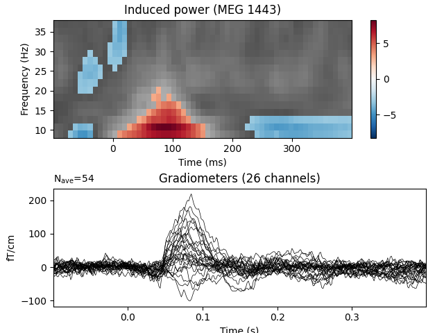
View time-frequency plots
evoked_data = evoked.data
times = 1e3 * evoked.times

plt.figure()
plt.subplots_adjust(0.12, 0.08, 0.96, 0.94, 0.2, 0.43)

# Create new stats image with only significant clusters
T_obs_plot = np.nan * np.ones_like(T_obs)
for c, p_val in zip(clusters, cluster_p_values):
    if p_val <= 0.05:
        T_obs_plot[c] = T_obs[c]

# Just plot one channel's data
ch_idx, f_idx, t_idx = np.unravel_index(
    np.nanargmax(np.abs(T_obs_plot)), epochs_power.shape[1:])
# ch_idx = tfr_epochs.ch_names.index('MEG 1332')  # to show a specific one

vmax = np.max(np.abs(T_obs))
vmin = -vmax
plt.subplot(2, 1, 1)
plt.imshow(T_obs[ch_idx], cmap=plt.cm.gray,
           extent=[times[0], times[-1], freqs[0], freqs[-1]],
           aspect='auto', origin='lower', vmin=vmin, vmax=vmax)
plt.imshow(T_obs_plot[ch_idx], cmap=plt.cm.RdBu_r,
           extent=[times[0], times[-1], freqs[0], freqs[-1]],
           aspect='auto', origin='lower', vmin=vmin, vmax=vmax)
plt.colorbar()
plt.xlabel('Time (ms)')
plt.ylabel('Frequency (Hz)')
plt.title(f'Induced power ({tfr_epochs.ch_names[ch_idx]})')

ax2 = plt.subplot(2, 1, 2)
evoked.plot(axes=[ax2], time_unit='s')
plt.show()
Total running time of the script: ( 0 minutes 13.359 seconds)
Estimated memory usage: 53 MB